Back to Portfolio of Projects | LearnableLoopAI.com | Blog |

In this project we establish an Active Inference (AIF) modeling approach making use of Bond Graphs, Generalized Filters, and Generalized Coordinates of Motion for traditional engineering systems. The emphasis will be on creating a framework and methodology, rather than applying it to a substantial problem. In this first part, we will make use of Bond Graphs to derive the state space equations that will be used in the following parts.

A few coding conventions:

Bold variable names usually start with an underscore, i.e. ’_’. That means all structured variables including vectors (i.e. tensors). The focus is on the code equivalents of the mathematics, i.e. not on Python structured variables, e.g. lists.
Global variable names (i.e. used across cells) are usually indicated by the Python ‘global’ keyword
External (i.e. true) states and parameters: The ‘^x’ symbol is used for code variables, i.e. ‘v^x’. In other words, superscript ‘x’ is used to imitate superscript ’*’ in code. In documentation the standard ‘ $v^{*}$ ’ is used.
This notebook follows a standardized framework. This is my own framework, developed over a number of years, and is informed by the CRISP-DM framework, the work of Warren Powell (Princeton), the work of Bert De Vries, the work of Karl Friston as well as that of the larger Active Inference community.

! python --version

Python 3.11.14

import matplotlib.pyplot as plt
import matplotlib.ticker as ticker
import numpy as np
import pandas as pd
from matplotlib.gridspec import GridSpec
from matplotlib.ticker import MaxNLocator

1 BUSINESS UNDERSTANDING

See Part 1

2 DATA UNDERSTANDING

N/A. We will not make use of collected data for training. Training happens online during simulation.

3 DATA PREPARATION

N/A. We will not make use of collected data for training. Training happens online during simulation.

4 MODELING

4.1 Narrative

4.2 Core Elements

This section attempts to answer three important questions:

What metrics are we going to track?
What decisions do we intend to make?
What are the sources of uncertainty?

Metrics

The temperature in the room relative to the control temperature will be tracked, $y (t)$

Decisions

The decision involves what control temperature should be injected into the room during each time step, $a_{1} (t)$

Sources of Uncertainty

A source of uncertainty is the outside temperature $v_{5} (t)$ . There is also uncertainty in the (colored) process and measurement noise.

4.3 System-Under-Steer / Environment / Generative Process

4.3.1 State variables

The state at time $t$ of the system-under-steer/environment (envir) is given by

$\begin{aligned} x_{t}^{*} & = (x_{t}^{StoredHeat}) & = (q_{3} (t)) \end{aligned}$ where

$q_{3} (t)$ : Heat stored in room by the $C_{3}$ thermal capacitor in J/K
- represented by the q3 code variable

4.3.2 Decision variables

The decision variables represent what we control.

The environment is steered by decisions/actions $a_{t}$ . Each component of this vector is called a control factor or control state factor. The action at time $t$ is given by

$\begin{aligned} a_{t} & = (a_{t}^{Temperature}) & = (a_{1} (t)) \end{aligned}$ where

$a_{1} (t)$ : Temperature applied by the HVAC system to the room in $^{\circ} C$
- represented by the a1 code variable

4.3.3 Exogenous information variables

The exogenous information is not controllable by the agent. $\begin{aligned} v_{t}^{*} & = (v_{t}^{OutsideTemperature}) & = (v_{5} (t)) \end{aligned}$

where

$v_{5} (t)$ : Outside Temperature in $^{\circ} C$
- represented by the v5 code variable

4.3.4 State Transition

To find the next state for each time step, the generative process starts with the transition function $f$ . To this is added system or process noise to arrive at the next state:

${\dot{x}}^{*} = f_{E} (x^{*}, v^{*}, a; θ_{x}^{*}) + ω_{x}^{*}$

4.3.5 Observation Generation

To find the observation generated by the external state of the generative process for each time step, the generative process starts with the generation function $g$ . To this is added observation or measurement noise to arrive at the observation:

$y = g_{E} (x^{*}, v^{*}, a; θ_{y}^{*}) + ω_{y}^{*}$

4.3.6 Implementation of the System-Under-Steer / Environment / Generative Process

$\begin{aligned} {\dot{x}}^{*} & = f_{E} (x^{*}, v^{*}, a; θ_{x}^{*}) + ω_{x}^{*} \\ {\dot{x}}_{0}^{*} & = - \frac{1}{C_{3} R_{6}} x_{0}^{*} + \frac{1}{R_{6}} v_{0}^{*} + \frac{1}{R_{6}} a_{0} + ω_{x}^{*} \\ {\dot{q}}_{3}^{*} (t) & = - \frac{1}{C_{3} R_{6}} q_{3}^{*} (t) + \frac{1}{R_{6}} v_{5}^{*} (t) + \frac{1}{R_{6}} a_{1} (t) + ω_{x}^{*} (t) \end{aligned}$

$\begin{aligned} y & = g_{E} (x^{*}, v^{*}; θ_{y}^{*}) + ω_{y}^{*} \\ y_{0} & = \frac{1}{C_{3}} x_{0}^{*} + ω_{y}^{*} \\ y (t) & = \frac{1}{C_{3}} q_{3}^{*} (t) + ω_{y}^{*} (t) \end{aligned}$

where

$x_{0}^{*}$ : Stored energy in room in J
- subscript 0 refers to the 0th component of the $x^{*}$ vector
$v_{0}^{*}$ : Outside temperature (exogenous force or disturbance) in $^{\circ} C$
- subscript 0 refers to the 0th component of the $v^{*}$ vector
$y_{0}^{*}$ : Room temperature in $^{\circ} C$
- subscript 0 refers to the 0th component of the $y$ vector
$ω_{x}^{*}$ : Process noise
$ω_{y}^{*}$ : Observation noise
$R_{6}$ : Thermal resistance between room and outside in K/W
$C_{3}$ : Thermal capacitance of the room in J/K
$θ_{x}^{*} = {R_{6}, C_{3}}$

ALPHA = 0.6
ENV_WIDTH = 4. ## 8.
AGT_WIDTH = 2.
AGT_LINESTYLES = ['-', '--', '-.', ':'] ## for agent
ORANGE_HUE_BY_SATURATION = [
    "#FFA500", ## 100% bright orange
    "#FFB347", ## 80% light vivid orange
    "#FFD580", ## 60% softer pastel orange
    "#FFE5B4"  ## 40% light faded orange
]
ORANGE_HUE_BY_BRIGHTNESS = [
    "#FFA500", ## 100% pure bright orange
    "#FFC04D", ## 80% light orange
    "#FFD699", ## 60% pastel orange
    "#FFE5CC"  ## 40% very pale orange
]
ORANGE_HUE = ORANGE_HUE_BY_BRIGHTNESS
styles = {
    #### envir
    "a": {
        "color": "crimson",
        "linestyle": "-",
        "linewidth": ENV_WIDTH,
        "alpha": ALPHA
    },
    "xˣ[0]": {
        "color": "black",
        "linestyle": "-",
        "linewidth": ENV_WIDTH,
        "alpha": ALPHA
    },
    "xˣ[1]": {
        "color": "darkgrey",
        "linestyle": "-",
        "linewidth": ENV_WIDTH,
        "alpha": ALPHA
    },
    "vˣ[0]": {
        "color": "blue",
        "linestyle": "-",
        "linewidth": ENV_WIDTH,
        "alpha": ALPHA
    },
    "vˣ[1]": {
        "color": "dodgerblue",
        "linestyle": "-",
        "linewidth": ENV_WIDTH,
        "alpha": ALPHA
    },
    "y[0]": {
        "color": ORANGE_HUE[0],
        "linestyle": "-",
        "linewidth": ENV_WIDTH,
        "alpha": ALPHA
    },
    "y[1]": {
        "color": ORANGE_HUE[1],
        "linestyle": "-",
        "linewidth": ENV_WIDTH,
        "alpha": ALPHA
    },
    "y[2]": {
        "color": ORANGE_HUE[2],
        "linestyle": "-",
        "linewidth": ENV_WIDTH,
        "alpha": ALPHA
    },
    "y[3]": {
        "color": ORANGE_HUE[3],
        "linestyle": "-",
        "linewidth": ENV_WIDTH,
        "alpha": ALPHA
    },
    #### agent
    "μ_x[0]": {
        "color": "black",
        "linestyle": AGT_LINESTYLES[0],
        "linewidth": AGT_WIDTH,
        "alpha": ALPHA
    },
    "μ_x[1]": {
        "color": "black",
        "linestyle": AGT_LINESTYLES[1],
        "linewidth": AGT_WIDTH,
        "alpha": ALPHA
    },
    "v[0]": {
        "color": "blue",
        "linestyle": AGT_LINESTYLES[0],
        "linewidth": AGT_WIDTH,
        "alpha": ALPHA
    },
    "v[1]": {
        "color": "blue",
        "linestyle": AGT_LINESTYLES[1],
        "linewidth": AGT_WIDTH,
        "alpha": ALPHA
    },
    "μ_v[0]": {
        "color": "dodgerblue",
        "linestyle": AGT_LINESTYLES[0],
        "linewidth": AGT_WIDTH,
        "alpha": ALPHA
    },
    "μ_v[1]": {
        "color": "dodgerblue",
        "linestyle": AGT_LINESTYLES[1],
        "linewidth": AGT_WIDTH,
        "alpha": ALPHA
    },
    "μ_y[0]": {
        "color": "orange", 
        "linestyle": AGT_LINESTYLES[0],
        "linewidth": AGT_WIDTH,
        "alpha": ALPHA
    },
    "μ_y[1]": {
        "color": "orange", 
        "linestyle": AGT_LINESTYLES[1],
        "linewidth": AGT_WIDTH,
        "alpha": ALPHA
    },
    "μ_y[2]": {
        "color": "orange", 
        "linestyle": AGT_LINESTYLES[2],
        "linewidth": AGT_WIDTH,
        "alpha": ALPHA
    },
    "F": {
        "color": "#9400D3", ## vivid deep violet
        "linestyle": "-",
        "linewidth": AGT_WIDTH,
        "alpha": ALPHA
    }
}

## Precision matrices
# def expand_diag(val, size):
#     return np.diag([val for _ in range(size)])

#### time
tT = 10000 ## end t in hours
Δt = 0.25 ## hours
ts = np.arange(0, tT, Δt) ## time steps
T = len(ts)

#### dimensionsionality of vectors
B = 1 ## number of dims for autonomous state vˣ/v
C = 1 ## number of dims for state xˣ/μ_x
D = 1 ## number of dims for observation y/μ_y
A = 1 ## number of dims for action a
M = 3 ## number of dims for embedding (generalized coordinates of motion)

#### noise
def white_noise(scale=1e-1, size=1):
    return np.random.normal(loc=0, scale=scale, size=size)
## white noise
σˣ2_x = 0.001
σˣ2_y = 0.001
_n_x = white_noise(scale=np.sqrt(σˣ2_x), size=(T,C))
_n_y = white_noise(scale=np.sqrt(σˣ2_y), size=(T,D))
## colored noise via AR(1) filters
_ω_x = np.zeros((T, C))
_ω_y = np.zeros((T, D))
α, β = 0.95, 0.10 ## process noise correlation
γ, δ = 0.90, 0.05 ## measurement noise correlation
## configure colored noise to be white again
## α, β = 0.00, 1.00 ## process noise correlation
## γ, δ = 0.00, 1.00 ## measurement noise correlation
for t in range(0, T - 1):
    _ω_x[t] = α*_ω_x[t-1] + β*_n_x[t]
    _ω_y[t] = γ*_ω_y[t-1] + δ*_n_y[t]

#### exogenous functions
def v_const(t, **kwargs):
    return kwargs['A']

def v_cos(t, **kwargs):
    return kwargs['A'] * np.cos(kwargs['θ1'] * t)

def v_pulses(t, **kwargs):
    """
    Sum of rectangular pulses defined in physical time.
    kwargs:
      'amps'   : list/array of amplitudes [A1, A2, ...]
      't_ons'  : list/array of start times [t_on1, t_on2, ...]
      't_offs' : list/array of end times   [t_off1, t_off2, ...]
    """
    amps   = np.asarray(kwargs['amps'], dtype=float)
    t_ons  = np.asarray(kwargs['t_ons'], dtype=float)
    t_offs = np.asarray(kwargs['t_offs'], dtype=float)
    t_arr = np.asarray(t, dtype=float)
    val = np.zeros_like(t_arr, dtype=float)
    for A, t_on, t_off in zip(amps, t_ons, t_offs):
        val += A * (np.heaviside(t_arr - t_on, 0.0) - np.heaviside(t_arr - t_off, 0.0))
    return float(val) if np.isscalar(t) else val

def v_lines(t, **kwargs):
    """
    Piecewise-linear signal defined by points (t_i, y_i).
    kwargs:
      't_pts' : list/array of time points [t0, t1, ..., tN]
      'y_pts' : list/array of values     [y0, y1, ..., yN]
    For t between t_i and t_{i+1}, returns the straight line
    interpolating between (t_i, y_i) and (t_{i+1}, y_{i+1}).
    For t < t0 returns y0, for t > tN returns yN.
    """
    t_pts = np.asarray(kwargs['t_pts'], dtype=float)
    y_pts = np.asarray(kwargs['y_pts'], dtype=float)
    if t_pts.ndim != 1 or y_pts.ndim != 1 or t_pts.size != y_pts.size:
        raise ValueError("t_pts and y_pts must be 1D arrays of the same length")
    t_arr = np.asarray(t, dtype=float)
    ## use numpy's 1D linear interpolation
    val = np.interp(t_arr, t_pts, y_pts)
    return float(val) if np.isscalar(t) else val

rng = np.random.default_rng(1234)
## --- Option 1: White Gaussian noise with std σ ---
def w_normal(t, **kwargs):
    ## t can be scalar or array; ignore its value, just match shape
    if np.isscalar(t):
        return kwargs['A'] * kwargs['sigma'] * rng.normal()
    else:
        return kwargs['A'] * kwargs['sigma'] * rng.normal(size=np.shape(t))
## --- Option 2: Uniform noise in [-A, A] ---
def w_uniform(t, **kwargs):
    ## rand in [0,1) → scale/shift to [-A, A]
    return (2 * kwargs['A']) * (rng.random() - 0.5)

## Disable noise for debugging
# _ω_x[:] = 0
# _ω_y[:] = 0
_ω_x[7], _ω_y[7]

(array([-0.00521211]), array([0.00350988]))

#### envir
θˣ_x = {
    'C3': 5.0,
    'R6': 2.0,
    'R_a': 1e-3 ## for now
}
def f_E(_xˣ, _vˣ, _a=[0], θˣ_x=θˣ_x): ## transition function for Envir
    C3 = θˣ_x['C3']
    R6 = θˣ_x['R6']
    q3 = _xˣ
    v5 = _vˣ[0]
    a1 = _a[0]
    t1_num = 1; t1_den = C3*R6
    t2_num = 1; t2_den = R6
    t3_num = 1; t3_den = R6
    dq3 = -(t1_num/t1_den)*q3 + (t2_num/t2_den)*v5 + (t3_num/t3_den)*a1 
    return [dq3] ## 1x1 matrix

def g_E(_xˣ, _vˣ=None): ## generation function for Envir
    q3 = _xˣ
    return np.array([
        (1 / θˣ_x['C3']) * q3 ## room temperature
    ])

def dy___da(_xˣ, _a, Δt, θˣ_x=θˣ_x):
    C3 = float(θˣ_x['C3'])
    R_a = float(θˣ_x['R_a']) ## whatever resistance couples a (temp) to the room
    return (Δt / (C3 * R_a)) ## scalar gain °C_out / °C_action

## disable noise for debugging
# _ω_x[:] = 0
# _ω_y[:] = 0
_ω_x[7], _ω_y[7]

(array([-0.00521211]), array([0.00350988]))

#### run
_a = np.zeros((T, A))
_xˣ = np.zeros((T, C))
_vˣ = np.zeros((T, B))
_y = np.zeros((T, D))

_a[0] = [0] ## aRoomTemperature
_xˣ[0] = [40] ## xˣRoomTemperature
_vˣ[0] = [-10] ## vˣOutdoorTemperature
_y[0] = [10] ## yRoomTemperature

v_funcs_env = {
    'a1': v_pulses,
    # 'v5': v_pulses,
    'v5': v_lines,
}
a1_theta_env = {
    'amps'  : [30., -30],
    't_ons' : [0., 5000],
    't_offs': [5000, 1e10],
}
# v5_theta_env = {
#     'amps'  : [7., -1.],
#     't_ons' : [0., 2500],
#     't_offs': [2500, 1e10],
# }
v5_theta_env = {
    'y_pts': [20, -3,    -9,   10],    
    't_pts' : [0., 2500, 5000, 10000],
}

for t in range(0, T - 1):
    _vˣ[t+1]  = v_funcs_env['v5'](ts[t], **v5_theta_env)
    ## vˣ[t+1] = sampled_vˣ ## vˣ[t+1] estimated from 1-step ahead historical data
    _a[t+1]  = v_funcs_env['a1'](ts[t], **a1_theta_env) ## estimated by using current observation from a sensor

    #### NEXT STATE
    _ẋ = f_E(_xˣ=_xˣ[t], _vˣ=_vˣ[t], _a=_a[t]) + _ω_x[t]
    _xˣ[t+1] = _xˣ[t] + _ẋ*Δt ## f is transition function; Euler
    
    #### OBSERVE
    _y[t+1] = g_E(_xˣ[t+1]) + _ω_y[t] ## g is generation function
result_env = pd.DataFrame({
    't': ts, 
    '_n_x_0': _n_x[:,0],
    '_ω_x_0': _ω_x[:,0],

    '_n_y_0': _n_y[:,0],
    '_ω_y_0': _ω_y[:,0],

    '_a_0': _a[:,0],
    '_xˣ_0': _xˣ[:,0], 
    '_vˣ_0': _vˣ[:,0], 
    '_y_0': _y[:,0]
})
print(result_env.head())
## print(result_env.iloc[40:60])

      t    _n_x_0    _ω_x_0    _n_y_0    _ω_y_0  _a_0      _xˣ_0    _vˣ_0  \
0  0.00  0.029897  0.002990  0.042808  0.002140   0.0  40.000000 -10.0000   
1  0.25 -0.005780  0.002262 -0.003945  0.001729   0.0  37.750747  20.0000   
2  0.50 -0.027086 -0.000559  0.000460  0.001579  30.0  39.307544  19.9977   
3  0.75 -0.007414 -0.001273  0.032516  0.003047  30.0  44.574428  19.9954   
4  1.00 -0.018758 -0.003085  0.006422  0.003063  30.0  49.709174  19.9931   

        _y_0  
0  10.000000  
1   7.552290  
2   7.863238  
3   8.916465  
4   9.944882

def plot_envir_result(result):
    ylabel_size = 12
    ylabelx = -0.3
    ylabely = 0.3
    fig = plt.figure(figsize=(10, 6))
    grid_rows = 8
    ## gs = GridSpec(grid_rows, 1, figure=fig, height_ratios=[3, 1, 1])
    gs = GridSpec(grid_rows, 1, figure=fig, height_ratios=[1]*grid_rows)
    ax = [fig.add_subplot(gs[i]) for i in range(grid_rows)]
    for j, axis in enumerate(ax):
        axis.set_xlim(0, tT)
        locator = MaxNLocator(nbins=5)
        axis.xaxis.set_major_locator(locator)
        axis.spines['top'].set_visible(False); axis.spines['right'].set_visible(False)
        if j < grid_rows - 1:
            axis.set_xticklabels([]) ## hide labels but keep tick positions

    i = 0
    ax[i].set_title(r'Environment', fontweight='bold',fontsize=14)
    ax[i].plot(result['t'], result['_a_0'], **styles['a'], label=r'$\mathbf{a}[0]=a_1(t)$: action temperature')
    ax[i].yaxis.set_label_coords(ylabelx, ylabely)
    ax[i].yaxis.set_major_formatter(ticker.EngFormatter(unit='$^{\\circ}\\mathrm{C}$'))
    ax[i].legend(loc='upper right')

    i += 1
    ax[i].plot(result['t'], result['_vˣ_0'], **styles['vˣ[0]'], label=r'$\mathbf{v}^*[0]=v_5(t)$: true outside temperature')
    ax[i].yaxis.set_label_coords(ylabelx, ylabely)
    ax[i].yaxis.set_major_formatter(ticker.EngFormatter(unit='$^{\\circ}\\mathrm{C}$'))
    ax[i].legend(loc='upper right')

    i += 1
    ax[i].plot(result['t'], result['_xˣ_0'], **styles['xˣ[0]'], label=r'$\mathbf{x}^*[0]=q_3(t)$: true room stored heat')
    ax[i].yaxis.set_label_coords(ylabelx, ylabely)
    ax[i].yaxis.set_major_formatter(ticker.EngFormatter(unit='J'))
    ax[i].legend(loc='upper right')

    i += 1
    ax[i].plot(result['t'], result['_y_0'], **styles['y[0]'], label=r'$\mathbf{y}[0]=y(t)$: obs room temperature')
    ax[i].yaxis.set_label_coords(ylabelx, ylabely)
    ax[i].yaxis.set_major_formatter(ticker.EngFormatter(unit='$^{\\circ}\\mathrm{C}$'))
    ax[i].legend(loc='upper right')

    i += 1 
    ax[i].plot(result['t'], result['_n_x_0'], color='black', linestyle=':', label=r'$n_x$')
    ax[i].yaxis.set_label_coords(ylabelx, ylabely)
    ax[i].yaxis.set_major_formatter(ticker.EngFormatter(unit='J'))
    ax[i].legend(loc='upper right')

    i += 1 
    ax[i].plot(result['t'], result['_ω_x_0'], color='black', linestyle=':', label=r'$ω_x$')
    ax[i].yaxis.set_label_coords(ylabelx, ylabely)
    ax[i].yaxis.set_major_formatter(ticker.EngFormatter(unit='J'))
    ax[i].legend(loc='upper right')

    i += 1 
    ax[i].plot(result['t'], result['_n_y_0'], color='orange', linestyle=':', label=r'$n_y$')
    ax[i].yaxis.set_label_coords(ylabelx, ylabely)
    ax[i].yaxis.set_major_formatter(ticker.EngFormatter(unit='$^{\\circ}\\mathrm{C}$'))
    ax[i].legend(loc='upper right')

    i += 1 
    ax[i].plot(result['t'], result['_ω_y_0'], color='orange', linestyle=':', label=r'$ω_y$')
    ax[i].yaxis.set_label_coords(ylabelx, ylabely)
    ax[i].yaxis.set_major_formatter(ticker.EngFormatter(unit='$^{\\circ}\\mathrm{C}$'))
    ax[i].legend(loc='upper right')

    ## bottom
    ticks = ax[-1].get_xticks()
    ax[-1].set_xticks(ticks)
    ## ax[-1].set_xticklabels([f"{1e6*t:.0f}" for t in ticks])  # micro-seconds
    ax[-1].set_xticklabels([f"{1e0*t:.0f}" for t in ticks])  # hours
    ax[i].set_xlabel('$\mathrm{Time}\ t\ [\mathrm{hours}]$', fontweight='bold', fontsize=12)
    ## plt.tight_layout()
    plt.subplots_adjust(hspace=0.3) ## Adjust this value as needed
    plt.show()
    fig.savefig("./ThermicSystem^v1-envir", bbox_inches="tight", dpi=300)
plot_envir_result(result_env)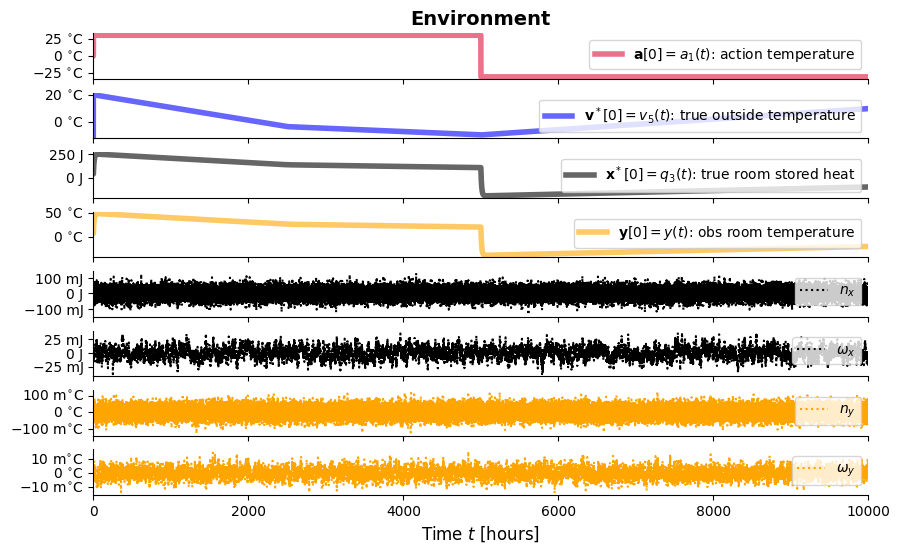

4.4 Uncertainty Model

As mentioned before, there is uncertainty in the (colored) process and measurement noise. We will also define models for the time behavior of the outside temperature $v_{5} (t)$ . We will experiment with step changes as well as daily cycles based on the cosine function.

4.5 AIF Agent / Generative Model

Quadratic/Laplace approximation

For some simplification in what follows, we make use of a quadratic approximation involving the application of a second order Taylor series expansion centered on the mean of the variational density $q (x)$ . Another assumption is that $q (x)$ is approximately Gaussian. This means we are effectively approximating the shape of $q (x)$ with a quadratic function at the second order of the Taylor series expansion. When $q (x)$ is sharply peaked or has high precision (low variance), this approximation is justified. This finally leads to the convenient property that the variance is a function of the mean:

$p (x ∣ y) \approx q_{μ_{x}, σ_{x}^{2}} (x) = N (x; μ_{x}, σ_{x}^{2}) \approx q_{μ_{x}} (x) = N (x; μ_{x}, σ_{x}^{2} (μ_{x}))$

The calculation of the variational density over the hidden state now only depends on the value of the mean. Effectively this is the same as assuming that $q (x)$ is a Dirac $δ$ function, but with the added advantage that we also get an approximation of the variance if we wish to find it.

Since the variational density is Gaussian and we plan to evaluate the function at the posterior mode, we substitute all occurences of $x$ in the generative model with $μ_{x}$ :

$\begin{aligned} \dot{x} & = f_{M} (μ_{x}, v; θ_{x}) + ω_{x} \\ {\dot{x}}_{0} & = - \frac{1}{C_{3} R_{6}} μ_{x 0} + \frac{1}{R_{6}} v_{0} + ω_{x} \\ {\dot{q}}_{3} (t) & = - \frac{1}{C_{3} R_{6}} q_{3} (t) + \frac{1}{R_{6}} v_{5} (t) + ω_{x} (t) \end{aligned}$

$\begin{aligned} y & = g_{M} (μ_{x}, v; θ_{y}) + ω_{y} \\ y_{0} & = \frac{1}{C_{3}} μ_{x 0} + ω_{y}^{*} \\ y (t) & = \frac{1}{C_{3}} q_{3} (t) + ω_{y}^{*} (t) \end{aligned}$

where

$μ_{x 0}$ : Mean of inferred stored energy in room in J
- subscript 0 refers to the 0th component of the $μ_{x}$ vector
$v_{0}$ : Inferred outside temperature (exogenous force or disturbance) in $^{\circ} C$
- subscript 0 refers to the 0th component of the $v$ vector
$y_{0}$ : Room temperature in $^{\circ} C$
- subscript 0 refers to the 0th component of the $y$ vector
$ω_{x}$ : Process noise
$ω_{y}$ : Observation noise
$R_{6}$ : Thermal resistance between room and outside in K/W
$C_{3}$ : Thermal capacitance of the room in J/K
$θ_{x}^{*} = {R_{6}, C_{3}}$

4.5.1 GF without generalized coordinates

#### agent
def f_M(_μₓ, _μᵥ):  # transition function for Model (agent)
    C3 = θˣ_x['C3']
    R6 = θˣ_x['R6']
    q3 = _μₓ
    v5 = _μᵥ
    t1_num = 1; t1_den = C3*R6
    t2_num = 1; t2_den = R6
    t3_num = 1; t3_den = R6
    dq3 = -(t1_num/t1_den)*q3 + (t2_num/t2_den)*v5
    return np.array([dq3]) ## 1x1 matrix

def g_M(_μₓ, _μᵥ=None): ## generation function for Model
    q3 = _μₓ
    return np.array([
        (1 / θˣ_x['C3']) * q3 ## room temperature
    ])    

def df_M___dμₓ(_μₓ, _μᵥ):
    C3 = θˣ_x['C3']
    R6 = θˣ_x['R6']
    return np.array([[-1.0 / (C3 * R6)]], dtype=float) ## shape (C, C)

def dg_M___dμₓ(_μₓ, _μᵥ):
    return np.array([[1 / θˣ_x['C3']]], dtype=float) ## shape (D, C)

def h_M(_μₓ, _μᵥ):
    ## setpoint on state: h_M(μₓ) = μₓ
    ## return μₓ ## shape (C,)

    ## setpoint on observation: h_M(μₓ) = g_M(μₓ)
    return g_M(_μₓ, _μᵥ) ## shape (D,)

def dh_M___dμₓ(_μₓ, _μᵥ):
    return np.array([[1 / θˣ_x['C3']]], dtype=float) ## shape (C, C)

## def dg_M___da(_μₓ, _a): ## direct action on observation (rare)
##     ## C is a matrix mapping action to observation
##     return C ## shape: (D, control_dim)
def dg_M___da(_μₓ, _a):
    ## If action appears directly in state, and observation is identity:
    return np.eye(D, A) ## shape (D, control_dim)
    ## If higher dimensional, tune dimensions.

#### run
_a = np.zeros((T, A)) ## action vector
_xˣ = np.zeros((T, C)) ## true state vector
_vˣ = np.zeros((T, B)) ## exogenous force vector
_y = np.zeros((T, D)) ## observation vector

_μ_x = np.zeros((T, C))

## _v = np.ones((T, C)) * [15.0] ## setpoints
_v = np.ones((T, D)) * [15.0] ## setpoints
## _μ_v = np.zeros((T, C)) * [15.0] ## setpoints; static, same as _v
_μ_v = np.zeros((T, D)) * [15.0] ## setpoints; static, same as _v

_μ_y = np.zeros((T, D)) ## expectation (belief) about y

_ϵ_x = np.zeros((T, C))
_ϵ_y = np.zeros((T, D))
## _ϵ_v = np.zeros((T, C))
_ϵ_v = np.zeros((T, D))

F = np.zeros(T) ## VFE
_dF___dμₓ = np.zeros((T, C))
_dF___da = np.zeros((T, A))

_a[0] = [0.] ## aRoomTemperature [C]
_xˣ[0] = [10.0] ## xˣRoomTemperature [C]
_vˣ[0] = [0.] ## vˣOutdoorTemperature [C]
_y[0] = [0.] ## yq3 [C]

_μ_x[0] = [0.0] ## μ_xq3 μ_xRoomTemperature ## initial state belief (before seeing data)
_μ_v[0] = [10.] ## μ_vOutdoorTemperature
_μ_y[0] = g_M(_μ_x[0], _μ_v[0]) ## μ_yRoomTemperature ## initial observation belief (before seeing data)

## _ϵ_x[0] = _μ_x[0] - f_M(_μₓ=_μ_x[0], _v=_μ_v[0]) ## initial model prediction error
_ϵ_x[0] = _μ_x[0] - f_M(_μ_x[0], _μ_v[0]) ## initial model prediction error; pass in vˣ
_ϵ_v[0] = h_M(_μ_x[0], _μ_v[0]) - _v[0]
_ϵ_y[0] = _y[0] - g_M(_μ_x[0], _μ_v[0]) ## initial sensory prediction error

## state precision
## _λ_x = [10.]
## _λ_x = [0.2, 0.2]
_Π_x = np.diag([5.0])
## _Π_x = np.diag([10.0, 10.0])
## setpoint precision
## _λ_v = [50.0]
_Π_v = np.diag([500.0])
## _Π_v = np.diag([50.0, 50.0])
## observation precision
## _λ_y = [10.0] 
_Π_y = np.diag([10.0])
## _Π_y = np.diag([10.0, 10.0])

κ  = .00002 #0.05             ## learning rate (perception) 
κₐ = .00005 #0.010             ## learning rate (action) 

## F[0] = 0.5 * ( _λ_y * _ϵ_y[0]**2 + _λ_x * _ϵ_x[0]**2 + np.log(_λ_y**-1 * _λ_x**-1) )
## F[0] = 0.5*(
##     sum( _λ_y[d] * _ϵ_y[0][d]**2 + np.log(_λ_y[d]**-1) for d in range(D) ) +\
##     sum( _λ_x[c] * _ϵ_x[0][c]**2 + np.log(_λ_x[c]**-1) for c in range(C) ) +\
##     sum(_λ_v[d] * (_μ_y[0][d] - _v[0][d])**2 for d in range(D)) ## for setpoint
## )
F[0] = 0.5 * ( ## numerically more stable with log, log(1/x) = -log(x); act only on the diag elements to avoid divide-by-zero RuntimeWarnings
    np.sum(_Π_y @ (_ϵ_y[0]**2)) - np.sum(np.log(np.diag(_Π_y))) +
    np.sum(_Π_x @ (_ϵ_x[0]**2)) - np.sum(np.log(np.diag(_Π_x))) +
    np.sum(_Π_v @ (_ϵ_v[0]**2)) - np.sum(np.log(np.diag(_Π_v)))
)
## F[0] = 500_000 ## plot looks better
v_funcs_agt_wout = {
    # 'v5': v_pulses,
    # 'v5': v_lines,
    'v5': v_cos,
}
# v5_theta_agt_wout = {
#     'amps'  : [7.,   -1.,  -3,   10],
#     't_ons' : [0.,   1000, 2000, 5000],
#     't_offs': [1000, 2000, 5000, 1e10],
# }
# v5_theta_agt_wout = {
#     'y_pts': [20, -3,    -9,   10],    
#     't_pts' : [0., 2500, 5000, 10000],
# }
v5_theta_agt_wout = {
    'A': 1.,    
    'θ1': .003,
}

for t in range(T - 1):
    _vˣ[t+1]  = v_funcs_agt_wout['v5'](ts[t], **v5_theta_agt_wout) ## vˣ[t+1] estimated by using current observation from a sensor

    #### NEXT STATE
    _ẋ = f_E(_xˣ[t], _vˣ[t], _a[t]) + _ω_x[t]
    _xˣ[t+1] = _xˣ[t] + _ẋ*Δt

    #### OBSERVE
    _y[t+1] = g_E(_xˣ[t+1]) + _ω_y[t] ## g is generation function

    #### INFER
    ### A. Calculate VFE gradient wrt μₓ (Eq6.8 ---> Eq6.16)
    ## _dF___dμₓ[t] = _λ_y * _ϵ_y[t] * dg_M___dμₓ(_μ_x[t]) + \
    ##                _λ_x * _ϵ_x[t] * df_M___dμₓ(_μ_x[t]) + \
    ##                _λ_v * _ϵ_v[t] * dh_M___dμₓ(_μ_x[t]) ## (Eq6.8+setpoint); Eq6.8 contains a minus ??
    ## _dF___dμₓ[t] = _Π_y @ _ϵ_y[t] @ dg_M___dμₓ(_μ_x[t]) +\
    ##                _Π_x @ _ϵ_x[t] @ df_M___dμₓ(_μ_x[t]) +\
    ##                _Π_v @ _ϵ_v[t] @ dh_M___dμₓ(_μ_x[t]) ## (Eq6.16+setpoint)
    _J_obsr = dg_M___dμₓ(_μ_x[t], _μ_v[t]) ## Jacobian shape (D,C)
    _J_proc = df_M___dμₓ(_μ_x[t], _μ_v[t]) ## Jacobian shape (C,C)
    _J_setp = dh_M___dμₓ(_μ_x[t], _μ_v[t]) ## Jacobian shape (C,C)    
    _dF___dμₓ[t] = _Π_y @ _ϵ_y[t] @ _J_obsr + _Π_x @ _ϵ_x[t] @ _J_proc + _Π_v @ _ϵ_v[t] @ _J_setp

    ### A. Calculate VFE gradient wrt a (Eq7.7 ---> )
    ## _dF___da[t] = _λ_y * _ϵ_y[t] * dy___da(_a[t]) ## Eq7.7 and Eq7.8
    ## _dF___da[t] = _λ_y * _ϵ_y[t]                   ## gradient wrt action
    _dF___da[t] = (_Π_y @ _ϵ_y[t]) * dy___da(_xˣ[t], _a[t], Δt) ## Eq7.7 and Eq7.8

    ### B. Define hidden state flow (Eq6.9 ---> Eq6.17)
    _μ̇ₓ = -κ*_dF___dμₓ[t]
    
    ### B. Define action flows (Eq7.5 ---> Eq7.31)
    _ȧ = -κₐ*_dF___da[t] ## Eq7.5

    ### C. Hidden state & inferred observation update (Eq6.9 ---> Eq6.17); Perception; Euler
    _μ_x[t+1] = _μ_x[t] + _μ̇ₓ*Δt ## Perceptual update (gradient descent)
    _μ_y[t+1] = g_M(_μₓ=_μ_x[t+1], _μᵥ=_μ_v[t+1])

    ### C. Control state update (Eq7.6); Perception; Euler
    _a[t+1] = _a[t] + _ȧ*Δt ## (Eq7.6) ## Action update (gradient descent)
    ## _a[t+1] = np.clip(_a[t+1], -5, 5) ## Clamp action to reasonable range
    ## _a[t+1] = 0.0 ## comment in to see what happens if no action/control 

    ### D. Recalculate prediction errors (Eq6.6 ---> Eq6.12)
    ## _ϵ_x[t+1] = _μ_x[t+1] - f_M(_μₓ=_μ_x[t+1], _v=_μ_v[t+1])
    _ϵ_x[t+1] = _μ_x[t+1] - f_M(_μₓ=_μ_x[t+1], _μᵥ=_μ_v[t+1]) ## # shape (C,); pass in vˣ
    _ϵ_y[t+1] = _y[t+1] - g_M(_μₓ=_μ_x[t+1], _μᵥ=_μ_v[t+1]) ## shape (D,)
    ## _ϵ_v[t+1] = h_M(_μₓ=_μ_x[t+1]) - _μ_v[t+1] ## shape (C,)
    _ϵ_v[t+1] = h_M(_μ_x[t+1], _μ_v[t+1]) - _v[t+1] ## (D,)
    
    ### E. Recalculate VFE (Eq6.7 --->  Eq6.15)
    ## F[t+1] = 0.5*( _λ_y * _ϵ_y[t+1]**2 + _λ_x * ϵ_x[t+1]**2 + np.log(_λ_y**-1 * _λ_x**-1) ) ## Eq6.7
    ## F[t+1] = 0.5*(
    ##     sum( _λ_y[d] * _ϵ_y[t+1][d]**2 + np.log(_λ_y[d]**-1) for d in range(D) ) +\
    ##     sum( _λ_x[c] * _ϵ_x[t+1][c]**2 + np.log(_λ_x[c]**-1) for c in range(C) ) +\
    ##     sum( _λ_v[d] * (_μ_y[t+1][d] - _v[t+1][d])**2 for d in range(D)) ## for setpoint
    ## ); #print(f'{F[t+1]=}')
    F[t+1] = 0.5*( ## numerically more stable with log, log(1/x) = -log(x); act only on the diag elements to avoid divide-by-zero RuntimeWarnings
        np.sum(_Π_y @ _ϵ_y[t+1]**2) - np.sum(np.log(np.diag(_Π_y))) +
        np.sum(_Π_x @ _ϵ_x[t+1]**2) - np.sum(np.log(np.diag(_Π_x))) +
        np.sum(_Π_v @ _ϵ_v[t+1]**2) - np.sum(np.log(np.diag(_Π_v)))
    )
result_agt = pd.DataFrame({
    't': ts, 
    '_a_0': _a[:,0],
    '_xˣ_0': _xˣ[:,0], 
    '_vˣ_0': _vˣ[:,0], 
    '_y_0': _y[:,0],
    '_v_0': _v[:,0],
    '_μ_x_0': _μ_x[:,0],
    '_μ_y_0': _μ_y[:,0],
    '_ϵ_x_0': _ϵ_x[:,0],
    '_ϵ_y_0': _ϵ_y[:,0],
    '_dF___dμₓ_0': _dF___dμₓ[:,0], 
    '_dF___da_0': _dF___da[:,0], 
    'F': F
})
print(result_agt.head())

      t      _a_0      _xˣ_0     _vˣ_0      _y_0  _v_0    _μ_x_0    _μ_y_0  \
0  0.00  0.000000  10.000000  0.000000  0.000000  15.0  0.000000  0.000000   
1  0.25  0.000000   9.750747  1.000000  1.952290  15.0  0.007488  0.001498   
2  0.50 -0.012192   9.632544  1.000000  1.928238  15.0  0.014967  0.002993   
3  0.75 -0.024225   9.515067  0.999999  1.904593  15.0  0.022447  0.004489   
4  1.00 -0.036101   9.398844  0.999997  1.882816  15.0  0.029925  0.005985   

     _ϵ_x_0    _ϵ_y_0  _dF___dμₓ_0  _dF___da_0             F  
0 -5.000000  0.000000 -1497.500000    0.000000  56307.436684  
1  0.008236  1.950792 -1495.952783  975.396192  56252.734119  
2  0.016464  1.925245 -1495.858398  962.622269  56241.021539  
3  0.024691  1.900103 -1495.763208  950.051622  56229.325375  
4  0.032918  1.876831 -1495.664290  938.415351  56217.672758

def plot_agent_result(result_agt):
    ylabel_size = 12
    ylabelx = -0.3
    ylabely = 0.3
    fig = plt.figure(figsize=(12, 22)) ## 2 inches/plot to get height
    grid_rows = 7
    ## gs = GridSpec(grid_rows, 1, figure=fig, height_ratios=[3, 1, 1, 1, 1, 1])
    gs = GridSpec(grid_rows, 1, figure=fig, height_ratios=[1]*grid_rows)
    ax = [fig.add_subplot(gs[i]) for i in range(grid_rows)]
    for j, axis in enumerate(ax):
        axis.grid(True)
        axis.set_xlim(0, tT)
        locator = MaxNLocator(nbins=5)
        axis.xaxis.set_major_locator(locator)
        axis.spines['top'].set_visible(False); axis.spines['right'].set_visible(False)
        if j < grid_rows - 1:
            axis.set_xticklabels([]) ## hide labels but keep tick positions

    i = 0
    ax[i].set_title(
        f'Agent\n' + r'(without generalized coordinates)', 
        fontweight='bold',fontsize=14)
    ax[i].plot(result_agt['t'], result_agt['_a_0'], **styles['a'], label=r'$\mathbf{a}[0]=a_1(t)$: action temperature')
    ax[i].yaxis.set_label_coords(ylabelx, ylabely)
    ax[i].yaxis.set_major_formatter(ticker.EngFormatter(unit='$^{\\circ}\\mathrm{C}$'))
    ax[i].legend(loc='upper left')

    i += 1
    ax[i].plot(result_agt['t'], result_agt['_vˣ_0'], **styles['vˣ[0]'], label=r'$\mathbf{v}^*[0]=v_5(t)$: true outside temperature')
    ax[i].yaxis.set_label_coords(ylabelx, ylabely)
    ax[i].yaxis.set_major_formatter(ticker.EngFormatter(unit='$^{\\circ}\\mathrm{C}$'))
    ax[i].legend(loc='upper left')

    i += 1
    ax[i].plot(result_agt['t'], result_agt['_xˣ_0'], **styles['xˣ[0]'], label=r'$\mathbf{x}^*[0]=q_3(t)$: true room stored heat')
    ax[i].plot(result_agt['t'], result_agt['_μ_x_0'], **styles['μ_x[0]'], label=r'$\boldsymbol{μ}_x[0]$: exp room stored heat')
    ax[i].yaxis.set_label_coords(ylabelx, ylabely)
    ax[i].yaxis.set_major_formatter(ticker.EngFormatter(unit='J'))
    ax[i].legend(loc='upper left')

    i += 1
    ax[i].plot(result_agt['t'], result_agt['_v_0'], **styles['v[0]'], label=r'$\mathbf{v}[0]=v(t)$: room temperature setpoint')
    ## ax[i].plot(result_agt['t'], result_agt['_μ_v_0'], **_styles['μ_v'], label=f'$μ_v$: exp outside temperature')
    ax[i].plot(result_agt['t'], result_agt['_y_0'], **styles['y[0]'], label=r'$\mathbf{y}[0]=y(t)$: obs room temperature')
    ax[i].plot(result_agt['t'], result_agt['_μ_y_0'], **styles['μ_y[0]'], label=r'$\mathbf{μ}_y[0]$: exp room temperature')
    ax[i].yaxis.set_label_coords(ylabelx, ylabely)
    ax[i].yaxis.set_major_formatter(ticker.EngFormatter(unit='$^{\\circ}\\mathrm{C}$'))
    ax[i].legend(loc='lower right')

    i += 1
    ax[i].plot(result_agt['t'], result_agt['_ϵ_x_0'], color='black', linestyle='-', label=r'$ϵ_{x}$')
    ax[i].plot(result_agt['t'], result_agt['_ϵ_y_0'], color='orange', linestyle='-', label=r'$ϵ_{y}$')
    ax[i].set_xticklabels([])
    ax[i].spines['top'].set_visible(False); ax[i].spines['right'].set_visible(False)
    ax[i].yaxis.set_label_coords(ylabelx, ylabely)
    ax[i].legend(loc='lower left')

    i += 1
    ax[i].plot(result_agt['t'], result_agt['_dF___dμₓ_0'], color='purple', linestyle='-', label=r'$\frac{dF}{dμ_{x0}}$')
    ax[i].plot(result_agt['t'], result_agt['_dF___da_0'], color='cyan', linestyle='-', label=r'$\frac{dF}{da_{0}}$')
    ax[i].set_xticklabels([])
    ax[i].spines['top'].set_visible(False); ax[i].spines['right'].set_visible(False)
    ax[i].yaxis.set_label_coords(ylabelx, ylabely)
    ax[i].legend(loc='upper right')

    i += 1
    ax[i].plot(result_agt['t'], result_agt['F'], color='red', linestyle='-', label=f'$\cal F$')
    ax[i].set_xticklabels([])
    ax[i].spines['top'].set_visible(False); ax[i].spines['right'].set_visible(False)
    ax[i].yaxis.set_label_coords(ylabelx, ylabely)
    ax[i].legend(loc='upper right')

    ## bottom
    ticks = ax[-1].get_xticks()
    ax[-1].set_xticks(ticks)
    ## ax[-1].set_xticklabels([f"{1e6*t:.0f}" for t in ticks])  # micro-seconds
    ax[-1].set_xticklabels([f"{1e0*t:.0f}" for t in ticks])  # hours
    ax[i].set_xlabel('$\mathrm{Time}\ t\ [\mathrm{hours}]$', fontweight='bold', fontsize=12)
    ## plt.tight_layout()
    plt.subplots_adjust(hspace=0.3) ## Adjust this value as needed
    plt.show()
    fig.savefig("./ThermicSystem^v1-agent-woutGC", bbox_inches="tight", dpi=300)
## plot_agent_result(result_agt)

from IPython.display import Image, display
display(Image(filename="ThermicSystem^v1-agent-woutGC-step.png"))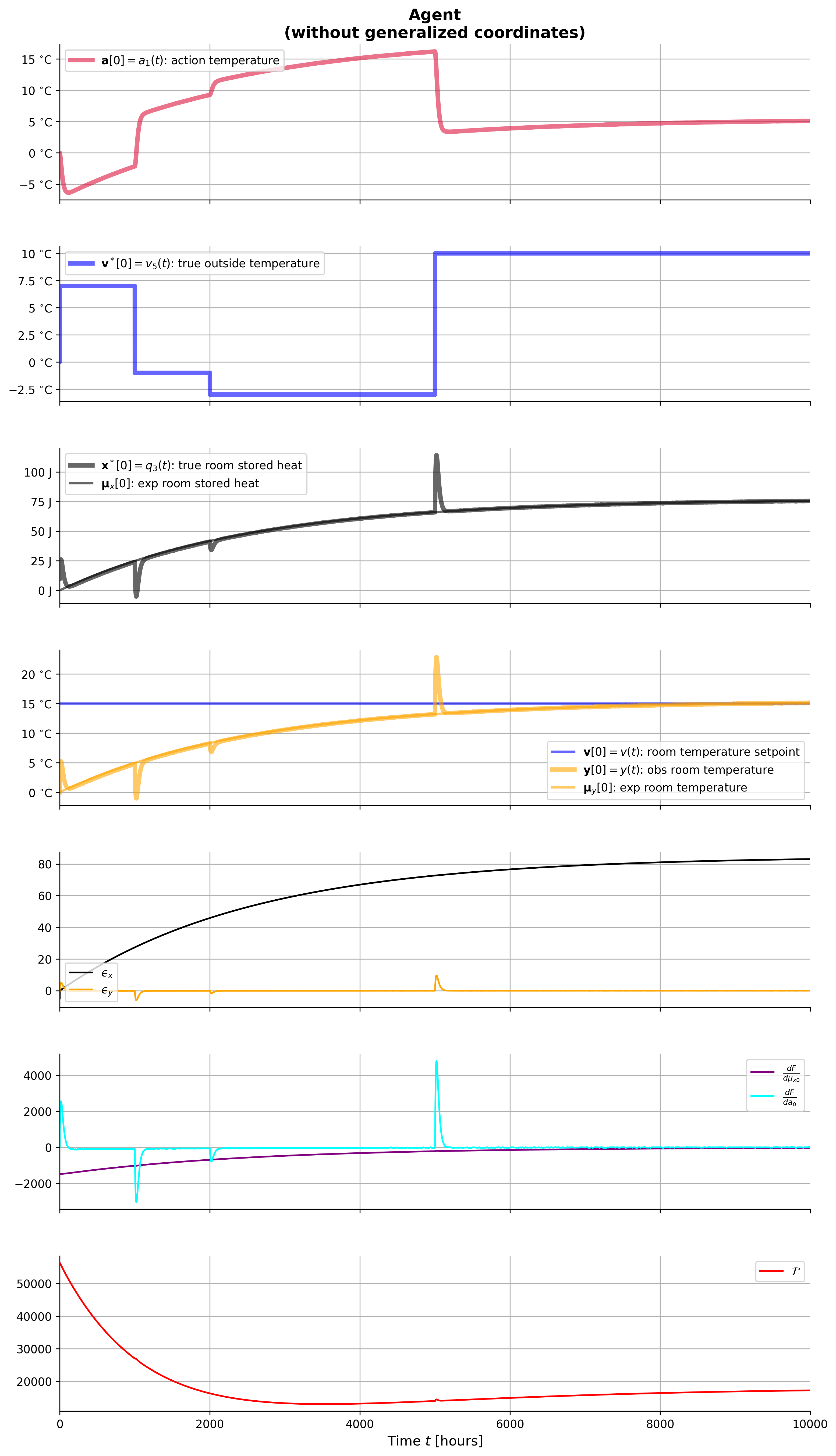

from IPython.display import Image, display
display(Image(filename="ThermicSystem^v1-agent-woutGC-ramp.png"))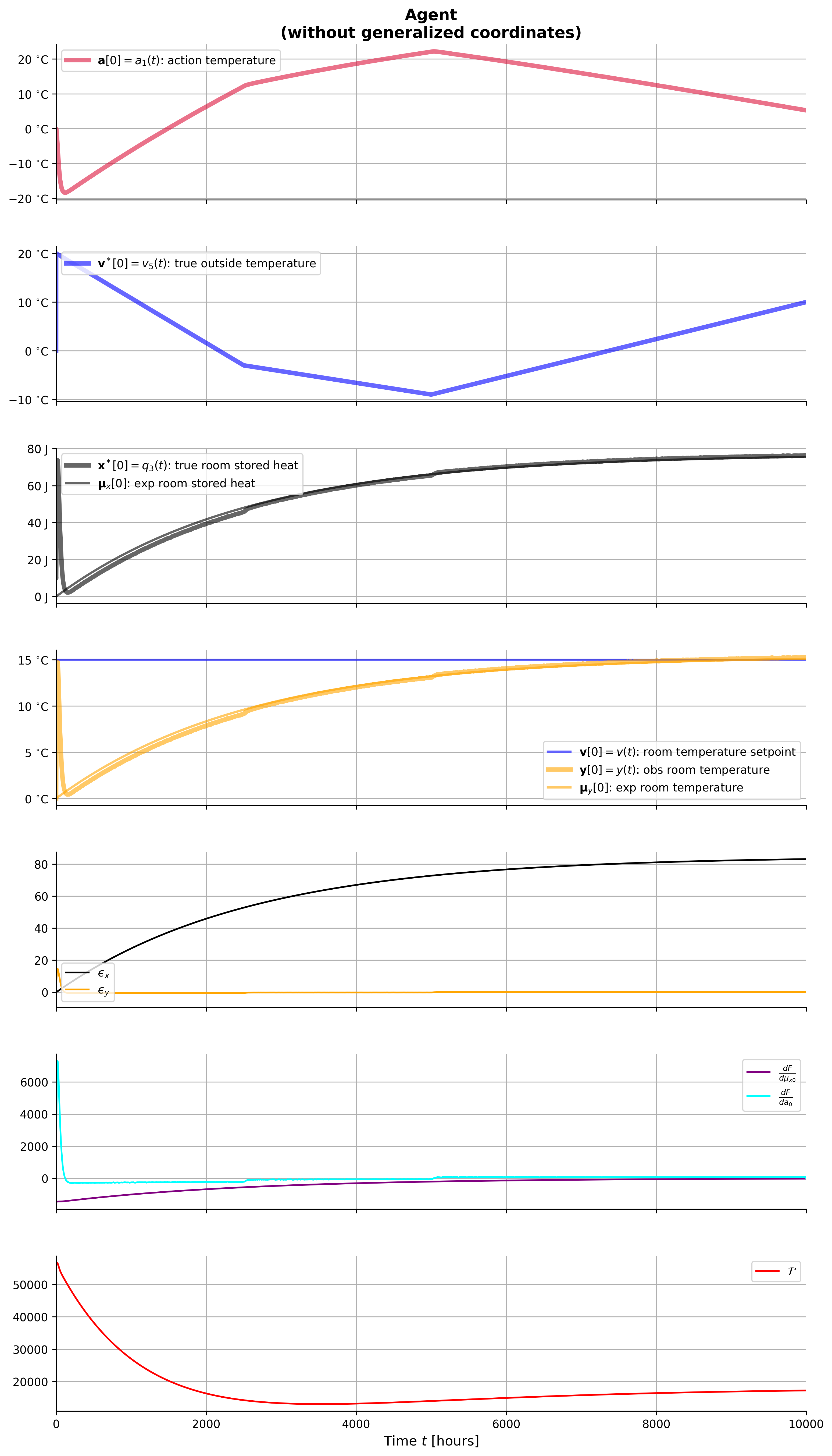

from IPython.display import Image, display
display(Image(filename="ThermicSystem^v1-agent-woutGC-cos.png"))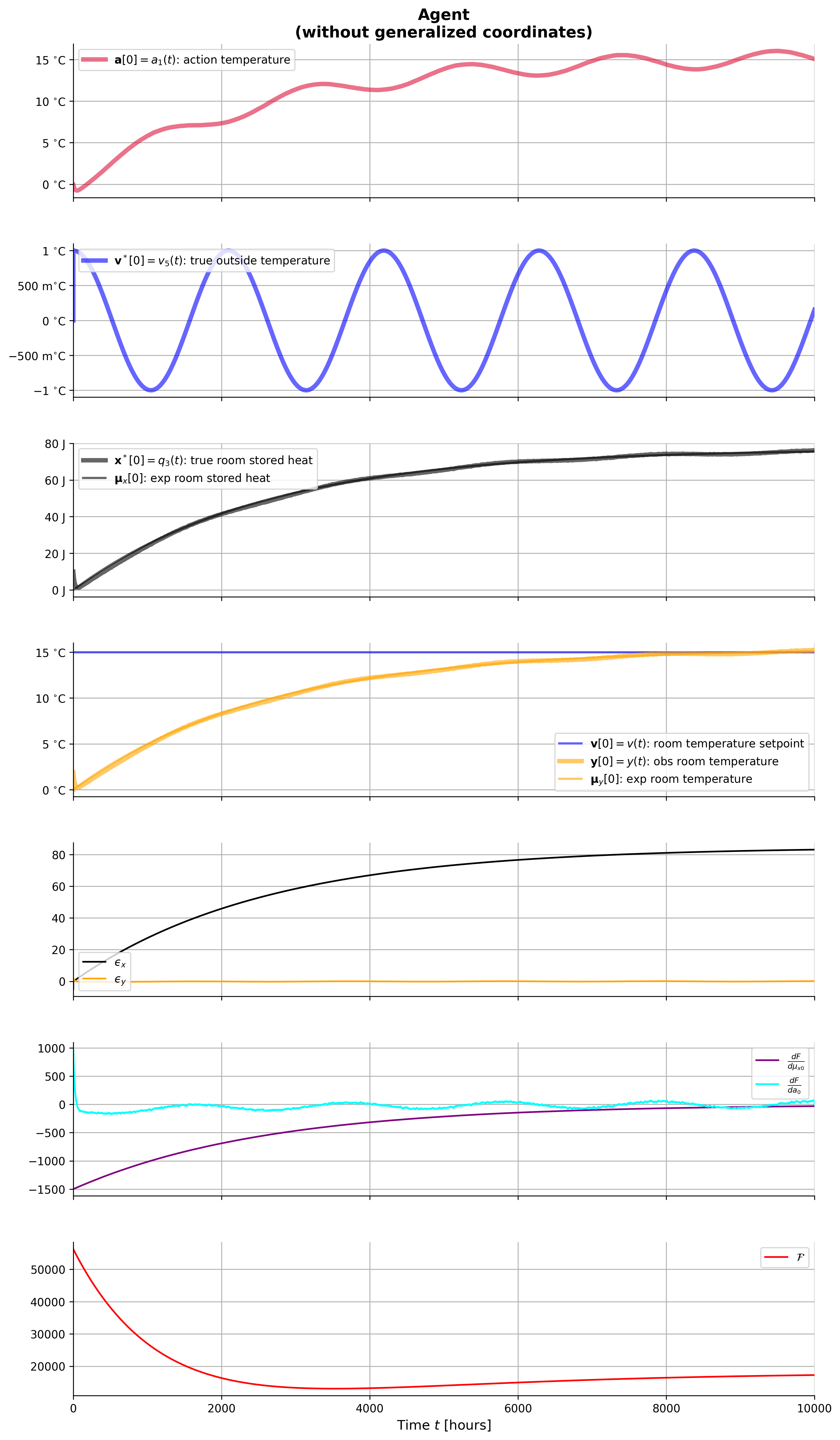

4.5.2 GF with generalized coordinates

def create_temporal_precision_matrix(M: int, γ: float, σ2: float) -> np.array:
    """ Creates a generalized precision matrix 
    Based on Matlab code from Hijne 2020, pp. 20-21.
    Creates a temporal covariance matrix for p+1 orders using a roughness of gamma for
    the amount of smoothening. The variance is then used to construct the generalized
    precision matrix.
    Args:
        M (int): The embedding order
        γ (float): Roughness parameter
        σ2 (float): Variance for x or y (i.e. σ2 * I)
    Returns:
        _np.array: The generalized precision matrix [M+1, M+1]
    """
    ## Order of the required autocorrelation derivatives
    k = np.arange(0, 2*M+1, 2)
    s = np.sqrt(2 / γ)
    ρ = np.cumprod(1-k) / (np.sqrt(2) * s)**k
    ρ = np.insert(arr=ρ, obj=np.arange(1,len(ρ), 1), values=0)
    ## Initialize temporal covariance matrix
    S = np.zeros((M+1, M+1))
    ## Loop over all rows of embedding order and population
    for r in range(0, M+1):
        S[r] = ρ[r:r+M+1]
        ρ = -ρ   # Inverse rho to alternate minus signs
    ## Compute generalized precision matrix
    Π̃ = np.linalg.inv(np.kron(S, σ2))

    ##. replace zeros and negative values with a small positive number instead of zero; 
    ##.   for np.log() on the elements later
    for i in range(Π̃.shape[0]):
        for j in range(Π̃.shape[1]):
            if Π̃[i,j] <= 0:
                Π̃[i,j] = 1e-10 ##. small positive number instead of zero; for np.log()
    return Π̃

def D_operator(M):
    return np.insert(np.insert(np.eye(M), 0, 0, axis=1), M, 0, axis=0)

## Works for C=1 (scalar state) and any C>1 without changes.
## Avoids any fixed indices like [_\mu_v[0], _\mu_v[3]]
## Lets you later change the initialization (e.g. mix \mu_x and \mu_v) by only modifying
##   the two lines that set _\mu_x_embedding[0, :] and [1, :], without touching the shape
###   logic
def embed_μ_x(_μ_x, _μ_v, M, C):
    """
    Embed state belief μ_x into generalized coordinates up to order M.
    _μ_x : array_like, shape (C,)
        Current state belief.
    _μ_v : array_like, shape (C,) or (D,) depending on your convention.
           Here we only use the components you choose to initialise with.
    M    : int
        Highest generalized order (0..M).
    C    : int
        State dimension.
    """
    _μ_x = np.asarray(_μ_x).reshape(C,)       ## ensure shape (C,)
    _μ_v = np.asarray(_μ_v).reshape(-1,)      ## 1‑D

    ## Process model and Jacobian
    _f  = f_M(_μ_x, _μ_v)                     ## shape (C,)
    _fp = df_M___dμₓ(_μ_x, _μ_v)              ## shape (C, C)

    ## Allocate embedding: rows = generalized order, cols = state components
    _μ_x_embedding = np.zeros((M + 1, C))

    ## 0th generalized coordinate: current state belief
    _μ_x_embedding[0, :] = _μ_x

    ## 1st generalized coordinate: state velocity
    _μ_x_embedding[1, :] = _f

    ## Higher‑order generalized coordinates: successive applications of Jacobian
    for i in range(2, M + 1):
        _μ_x_embedding[i, :] = _fp @ _μ_x_embedding[i - 1, :]

    return _μ_x_embedding

def embed_y(_y, _x, _v, M, C, D):
    _f = f_M(_x, _v)
    _fp = df_M___dμₓ(_x, _v)
    _g = g_M(_x, _v)
    _gp = dg_M___dμₓ(_x, _v)
    _x_embedding = np.zeros((M+1, C))
    _y_embedding = np.zeros((M+1, D))
    _x_embedding[0] = _f
    for i in range(1, M+1): ## propagate with Jacobian for higher-order terms
        _x_embedding[i] = _fp @ _x_embedding[i-1]
    _y_embedding[0] = _g
    for i in range(1, M+1):
        _y_embedding[i] = _gp @ _x_embedding[i-1]
    return _y_embedding

def embed_func(func, dfunc, _μ̃_x, _μ_v, dim):
    M = _μ̃_x.shape[0] - 1
    _func_vec = np.zeros((M+1, dim))
    _motion_vec = np.ones((M+1, dim))
    _func_vec[0] = 1
    _motion_vec[0] = 0
    _jac = dfunc(_μ̃_x[0], _μ_v) ## shape (C, C)
    ## Apply Jacobian to each embedded coordinate
    _motion_term = np.array([_jac @ _μ̃_x[m] for m in range(M+1)]) ## (M+1, C)
    _f̃ = _func_vec * func(_μ̃_x[0], _μ_v[0]) + _motion_term
    return _f̃

#### run
## tuning very sensitive to κ, λ_x, λ_y
_a = np.zeros((T, A)) ## action vector
_xˣ = np.zeros((T, C)) ## true state vector
_vˣ = np.zeros((T, B)) ## exogenous force vector
_y = np.zeros((T, D))  ## observation vector
_ỹ   = np.zeros((T, M+1, D)) ## generalized sensory input

_μ_x = np.zeros((T, C))
_μ̃_x = np.zeros((T, M+1, C)) ## generalized expectation of x
## _v = np.ones((T, C)) * [15.0] ## setpoints
_v = np.ones((T, D)) * [15.0] ## setpoints
_μ_v = np.ones((T, D)) * [15.0] ## setpoints; static, same as _v
_μ̃_v = np.zeros((T, M+1, D)) ## generalized expected or 'desired' hidden state

_μ_y = np.zeros((T, D)) ## expectation (belief) about y
_μ̃_y = np.zeros((T, M+1, D)) ## NEW

## _ϵ_x = np.zeros((T, C))
## _ϵ_y = np.zeros((T, D))
_ϵ̃_x = np.zeros((T, M+1, C))
_ϵ̃_v = np.zeros((T, M+1, D))
_ϵ̃_y = np.zeros((T, M+1, D)) ## Generalized p.e. [t, 2(M+1), 1]

F = np.zeros(T) ## VFE
## _dF___dμₓ = np.zeros((T, C))
_dF___dμ̃ₓ = np.zeros((T, M+1, C))
_dF___da = np.zeros((T, A))

_a[0] = [0.] ## aRoomTemperature [C]
_xˣ[0] = [10.0] ## xˣRoomTemperature [C]
_vˣ[0] = [0.] ## vˣOutdoorTemperature [C]
_y[0] = [0.] ## yq3 [C]
_ỹ[0] = embed_y(_y=_y[0], _x=_xˣ[0], _v=_vˣ[0], M=M, C=C, D=D)

## _μ_x[0] = [15, 7] ## initial state belief (before seeing data)
_μ_x[0] = [15] ## μ_xRoomTemperature  ## initial state belief (before seeing data)
## _μ_v[0] = [10, 15]
_μ_v[0] = [10] ## μ_vOutdoorTemperature
_μ̃_x[0] = embed_μ_x(_μ_x[0], _μ_v[0], M, C); print(f'{_μ̃_x[0]=}')
_μ_y[0] = g_M(_μ_x[0], _μ_v[0]) ## μ_yRoomTemperature ## initial observation belief (before seeing data)

Dop = D_operator(M); print(f'{Dop=}')  ## D operator for _M = 3

## _ϵ_x[0] = _μ_x[0] - f_M(_μ_x[0]) ## initial model prediction error
## _ϵ_y[0] = _y[0] - g_M(_μ_x[0]) ## initial sensory prediction error
_ϵ̃_x[0] = Dop @ _μ̃_x[0] - embed_func(f_M, df_M___dμₓ, _μ̃_x[0,:], _μ̃_v[0,:], C)
## _ϵ̃_v[0] = Dop @ _μ̃_x[0] - embed_func(h_M, dh_M___dμₓ, _μ̃_x[0,:], _μ̃_v[0,:], C)
_ϵ̃_v[0] = _ỹ[0] - _μ̃_v[0]
_ϵ̃_y[0] = _ỹ[0]        - embed_func(g_M, dg_M___dμₓ, _μ̃_x[0], _μ̃_v[0], D)

γ_x = 1e4 ## roughness x
γ_y = 1e4 ## roughness y
γ_v = 1e4 ## roughness v
λ_x = 1/2 ## Prior precision
## _Π_x = np.diag([10.0])
λ_y = 1/2 ## Likelihood precision
## _Π_y = np.diag([10.0])
λ_v = 1/2 ## Setpoint precision
_Π̃_x = create_temporal_precision_matrix(M=M, γ=γ_x, σ2=1/λ_x)
_Π̃_y = create_temporal_precision_matrix(M=M, γ=γ_y, σ2=1/λ_y)
_Π̃_v = create_temporal_precision_matrix(M=M, γ=γ_v, σ2=1/λ_v)

κ = 1  # 1 .01 .1 1                 ## learning rate (perception)
κₐ = 5e-5 ## .00005 # .00001 0.010  ## learning rate (action) 
Π_v0 = .64 ## .1  # tuning scalar

F[0] = 0.5 * ( ## Eq6.55+actions
    sum(
        _Π̃_y[m, d] * _ϵ̃_y[0][m, d]**2 + np.log(_Π̃_y[m, d])
        for d in range(D)
        for m in range(M+1)
    ) +
    sum(
        _Π̃_x[m, c] * _ϵ̃_x[0][m, c]**2 + np.log(_Π̃_x[m, c])
        for c in range(C)
        for m in range(M+1)
    ) +
    sum(
        _Π̃_v[m, c] * _ϵ̃_v[0][m, c]**2 + np.log(_Π̃_v[m, c])
        for c in range(C)
        for m in range(M+1)
    )
)
## F[0] = 100 ## makes plot look better
v_funcs_agt_with = {
    # 'v5': v_pulses,
    # 'v5': v_lines,
    'v5': v_cos,
}
# v5_theta_agt_with = {
#     'amps'  : [7.,   -1.,  -3,   10],
#     't_ons' : [0.,   1000, 2000, 5000],
#     't_offs': [1000, 2000, 5000, 1e10],
# }
# v5_theta_agt_with = {
#     'y_pts': [20, -3,    -9,   10],    
#     't_pts' : [0., 2500, 5000, 10000],
# }
v5_theta_agt_with = {
    'A': 1.,    
    'θ1': .003,
}

for t in range(T - 1):
    _vˣ[t+1]  = v_funcs_agt_with['v5'](ts[t], **v5_theta_agt_with) ## vˣ[t+1] estimated by using current observation from a sensor

    #### NEXT STATE
    _ẋ = f_E(_xˣ=_xˣ[t], _vˣ=_vˣ[t], _a=_a[t]) + _ω_x[t]
    _xˣ[t+1] = _xˣ[t] + _ẋ*Δt
    
    #### OBSERVE
    _y[t+1] = g_E(_xˣ[t+1]) + _ω_y[t] ## g is generation function

    #### INFER
    ### A. Calculate VFE gradient wrt μₓ (Eq6.8 ---> Eq6.16 ---> Eq6.62 and 6.63)
    ## _dF___dμₓ[t] = _Π_y @ _ϵ_y[t] @ dg_M___dμₓ(_μ_x[t]) + _Π_x @ _ϵ_x[t] @ df_M___dμₓ(_μ_x[t])
    Dop = D_operator(M)
    _dϵ̃___dμ̃_x = C*Dop - np.sum(df_M___dμₓ(_μ̃_x[t+1, 0, :], _μ̃_v[t+1, 0, :])) * np.eye(M+1)
    _dϵ̃___dμ̃_y = np.sum(dg_M___dμₓ(_μ̃_x[t+1, 0, :], _μ̃_v[t+1, 0, :])) * np.eye(M+1)
    # /////////////////////////////////////
    ## _dF___dμ̃ₓ[t] = _dϵ̃___dμ̃_x.T @ _Π̃_x @ _ϵ̃_x[t]   -   _dϵ̃___dμ̃_y.T @ _Π̃_y @ _ϵ̃_y[t] ## Eq6.63
    alpha_v_state = 2e-3 ## 1e-3   # start very small
    dh = np.sum(dh_M___dμₓ(_μ̃_x[t,0,:], _μ̃_v[t,0,:])) ## scalar ∂h/∂μ_x
    _dϵ̃_v_dμ̃x = dh * np.eye(M+1)  # (M+1, M+1)
    _dF___dμ̃ₓ[t] = ( ## Eq6.63
          _dϵ̃___dμ̃_x.T @ _Π̃_x @ _ϵ̃_x[t]
        - _dϵ̃___dμ̃_y.T @ _Π̃_y @ _ϵ̃_y[t]
        + alpha_v_state * (_dϵ̃_v_dμ̃x.T @ _Π̃_v @ _ϵ̃_v[t])
    )    
    # \\\\\\\

    ### A. Calculate VFE gradient wrt a (Eq7.7 ---> )
    # /////////////////////////////
    ## _dF___da[t] = _λ_y * _ϵ_y[t] * dy___da(a[t]) ## Eq7.7 and Eq7.8
    eps_y_gen = _ϵ̃_y[t, :, 0]              ## (M+1,)
    w_eps_y   = _Π̃_y @ eps_y_gen           ## (M+1,)
    dF_da_y   = w_eps_y[0] * dy___da(_xˣ[t], _a[t], Δt) ## scalar

    eps_v0    = _μ_y[t, 0] - _v[t, 0]       ## scalar
    dF_da_v   = Π_v0 * eps_v0 * dy___da(_xˣ[t], _a[t], Δt) ## scalar

    _dF___da[t] = np.array([dF_da_y + dF_da_v]) ## shape (1,)
    # \\\\\\\\\\

    ### B. Define hidden state flow (Eq6.9 ---> Eq6.17 ---> Eq6.64)
    ## _μ̇ₓ = κ*_dF___dμₓ[t]
    _μ̃̇ₓ = Dop @ _μ̃_x[t] - κ*_dF___dμ̃ₓ[t] ## Eq6.64

    ### B. Define action flows (Eq7.5 ---> Eq7.31)
    _ȧ = -κₐ*_dF___da[t] ## Eq7.5

    ### C. Hidden state & inferred observation update (Eq6.9 ---> Eq6.17 ---> Eq6.66); Perception; Euler
    ## _μ_x[t+1] = _μ_x[t] + _μ̇ₓ*_Δt
    ## _μ_y[t+1] = g_M(_μₓ=_μ_x[t+1], _v=_μ_v[t+1])
    _μ̃_x[t+1] = _μ̃_x[t] + _μ̃̇ₓ * Δt ## Eq6.66
    _ỹ[t+1] = embed_y(_y=_y[t+1], _x=_xˣ[t+1], _v=_vˣ[t+1], M=M, C=C, D=D)
    _μ_x[t+1] = _μ̃_x[t+1, 0]
    _μ_y[t+1] = g_M(_μ_x[t+1], _μ_v[t+1])
    
    ### C. Action update (Eq7.6); Perception; Euler
    _a[t+1] = _a[t] + _ȧ*Δt ## (Eq7.6) ## Action update (gradient descent)
    ## _a[t+1] = np.clip(_a[t+1], -5, 5) ## Clamp action to reasonable range
    ## _a[t+1] = 0.0 ## comment in to see what happens if no action/control 

    ### D. Recalculate prediction errors (Eq6.6 ---> Eq6.12 ---> Eq6.56 and 6.57)
    ## _ϵ_x[t+1] = _μ_x[t+1] - f_M(_μₓ=_μ_x[t+1], _v=_μ_v[t+1])
    ## _ϵ_y[t+1] = _y[t+1] - g_M(_μₓ=_μ_x[t+1], _v=_μ_v[t+1])
    _ϵ̃_x[t+1] = Dop @ _μ̃_x[t+1] - embed_func(f_M, df_M___dμₓ, _μ̃_x[t+1], _μ̃_v[t+1], C)
    _ϵ̃_y[t+1] = _ỹ[t+1]        - embed_func(g_M, dg_M___dμₓ, _μ̃_x[t+1], _μ̃_v[t+1], D)
    # ////////////////////////////////
    ## _ϵ̃_v[t+1] = Dop @ _μ̃_x[t+1] - embed_func(h_M, dh_M___dμₓ, _μ̃_x[t+1,:], _μ̃_v[t+1,:], C)
    ## generalized desired observation (here only order 0 non-zero)
    _μ̃_v[t+1, 0, 0] = _v[t+1, 0] # 15°C trajectory # desired temperature
    _μ̃_v[t+1, 1:, 0] = 0.0    
    _ϵ̃_v[t+1] = _μ̃_y[t+1] - _μ̃_v[t+1]  # belief about y vs desired y, all orders
    ## To make this meaningful, also maintain a generalized belief over y:
    ##   (can refine higher orders later if needed).
    _μ̃_y[t+1, 0, 0] = _μ_y[t+1, 0]
    _μ̃_y[t+1, 1:, 0] = 0.0
    # \\\\\\\\        

    ### E. Recalculate VFE (Eq6.7 --->  Eq6.15 ---> Eq6.55 or Eq6.75)
    F[t+1] = 0.5 * ( ## Eq6.55+actions
        sum(
            _Π̃_y[m, d] * _ϵ̃_y[t+1][m, d]**2 + np.log(_Π̃_y[m, d])
            for d in range(D)
            for m in range(M+1)
        ) +
        sum(
            _Π̃_x[m, c] * _ϵ̃_x[t+1][m, c]**2 + np.log(_Π̃_x[m, c])
            for c in range(C)
            for m in range(M+1)
        ) +
        sum(
            _Π̃_v[m, c] * _ϵ̃_v[t+1][m, c]**2 + np.log(_Π̃_v[m, c])
            for c in range(C)
            for m in range(M+1)
        )
    )
result_agt = pd.DataFrame({
    't': ts, 
    '_a_0': _a[:,0],
    '_xˣ_0': _xˣ[:,0], 
    '_vˣ_0': _vˣ[:,0], 
    '_y_0': _y[:,0],
    '_v_0': _v[:,0],

    '_μ_x_0': _μ_x[:,0],
    '_μ_v_0': _μ_v[:,0],
    '_μ_y_0': _μ_y[:,0],

    '_μ̃_x_1_0': _μ̃_x[:,1,0],
    '_μ̃_x_2_0': _μ̃_x[:,2,0],
    '_μ̃_x_3_0': _μ̃_x[:,3,0],

    '_ϵ̃_x_0_0': _ϵ̃_x[:,0,0],

    '_ϵ̃_y_0_0': _ϵ̃_y[:,0,0],

    '_dF___dμ̃ₓ_0_0': _ϵ̃_x[:,0,0],

    'F': F
})
print(result_agt.head())

_μ̃_x[0]=array([[15.   ],
       [ 3.5  ],
       [-0.35 ],
       [ 0.035]])
Dop=array([[0., 1., 0., 0.],
       [0., 0., 1., 0.],
       [0., 0., 0., 1.],
       [0., 0., 0., 0.]])
      t      _a_0      _xˣ_0     _vˣ_0      _y_0  _v_0     _μ_x_0  _μ_v_0  \
0  0.00  0.000000  10.000000  0.000000  0.000000  15.0  15.000000    10.0   
1  0.25  0.006675   9.750747  1.000000  1.952290  15.0  15.602975    15.0   
2  0.50  0.013438   9.633379  1.000000  1.928405  15.0  15.891975    15.0   
3  0.75  0.020243   9.519084  0.999999  1.905396  15.0  15.924517    15.0   
4  1.00  0.027063   9.408319  0.999997  1.884711  15.0  15.750335    15.0   

     _μ_y_0  _μ̃_x_1_0  _μ̃_x_2_0  _μ̃_x_3_0  _ϵ̃_x_0_0  _ϵ̃_y_0_0  \
0  3.000000   3.500000  -0.350000   0.035000   6.500000  -4.000000   
1  3.120595   2.193728  -0.341286   0.034837   5.314323  -4.291041   
2  3.178395   1.111959  -0.332596   0.034705   4.290354  -4.430114   
3  3.184903   0.224363  -0.323925   0.034597   3.409266  -4.465990   
4  3.150067  -0.495855  -0.315269   0.034512   2.654212  -4.418470   

   _dF___dμ̃ₓ_0_0          F  
0        6.500000 -59.980836  
1        5.314323  18.546059  
2        4.290354  15.312807  
3        3.409266  12.888475  
4        2.654212  11.013307

def plot_agent_result(result_agt):
    ylabel_size = 12
    ylabelx = -0.3
    ylabely = 0.3
    fig = plt.figure(figsize=(12, 22)) ## 2 inches/plot to get height
    grid_rows = 7
    ## gs = GridSpec(grid_rows, 1, figure=fig, height_ratios=[3, 1, 1, 1, 1, 1, 1, 1, 1])
    gs = GridSpec(grid_rows, 1, figure=fig, height_ratios=[1]*grid_rows)
    ax = [fig.add_subplot(gs[i]) for i in range(grid_rows)]
    for j, axis in enumerate(ax):
        axis.grid(True)
        axis.set_xlim(0, tT)
        locator = MaxNLocator(nbins=5)
        axis.xaxis.set_major_locator(locator)
        axis.spines['top'].set_visible(False); axis.spines['right'].set_visible(False)
        if j < grid_rows - 1:
            axis.set_xticklabels([]) ## hide labels but keep tick positions

    i = 0
    ax[i].set_title(
        f'Agent\n' + r'(with generalized coordinates)', 
        fontweight='bold',fontsize=14)
    ax[i].plot(result_agt['t'], result_agt['_a_0'], **styles['a'], label=r'$\mathbf{a}[0]=a_1(t)$: action temperature')
    ax[i].yaxis.set_label_coords(ylabelx, ylabely)
    ax[i].yaxis.set_major_formatter(ticker.EngFormatter(unit='$^{\\circ}\\mathrm{C}$'))
    ax[i].legend(loc='upper left')
    
    i += 1
    ax[i].plot(result_agt['t'], result_agt['_vˣ_0'], **styles['vˣ[0]'], label=r'$\mathbf{v}^*[0]=v_5(t)$: true outside temperature')
    ax[i].yaxis.set_label_coords(ylabelx, ylabely)
    ax[i].yaxis.set_major_formatter(ticker.EngFormatter(unit='$^{\\circ}\\mathrm{C}$'))
    ax[i].legend(loc='upper left')

    i += 1
    ax[i].plot(result_agt['t'], result_agt['_xˣ_0'], **styles['xˣ[0]'], label=r'$\mathbf{x}^*[0]=q_3(t)$: true room stored heat')
    ax[i].plot(result_agt['t'], result_agt['_μ_x_0'], **styles['μ_x[0]'], label=r'$\boldsymbol{μ}_x[0]$: exp room stored heat')
    ax[i].yaxis.set_label_coords(ylabelx, ylabely)
    ax[i].yaxis.set_major_formatter(ticker.EngFormatter(unit='J'))
    ax[i].legend(loc='upper left')

    i += 1
    ax[i].plot(result_agt['t'], result_agt['_v_0'], **styles['v[0]'], label=r'$\mathbf{v}[0]=v(t)$: room temperature setpoint')
    ## ax[i].plot(result_agt['t'], result_agt['_μ_v_0'], **_styles['μ_v'], label=f'$μ_v$: exp outside temperature')
    ax[i].plot(result_agt['t'], result_agt['_y_0'], **styles['y[0]'], label=r'$\mathbf{y}[0]=y(t)$: obs room temperature')
    ax[i].plot(result_agt['t'], result_agt['_μ_y_0'], **styles['μ_y[0]'], label=r'$\mathbf{μ}_y[0]$: exp room temperature')
    ax[i].yaxis.set_label_coords(ylabelx, ylabely)
    ax[i].yaxis.set_major_formatter(ticker.EngFormatter(unit='$^{\\circ}\\mathrm{C}$'))    
    ax[i].legend(loc='lower right')

    i += 1
    ax[i].plot(result_agt['t'], result_agt['_ϵ̃_x_0_0'], color='black', linestyle='-', label=r'$ϵ̃_{x00}$')
    ax[i].plot(result_agt['t'], result_agt['_ϵ̃_y_0_0'], color='orange', linestyle='-', label=r'$ϵ̃_{y00}$')
    ax[i].yaxis.set_label_coords(ylabelx, ylabely)
    ax[i].legend(loc='upper right')

    i += 1
    ax[i].plot(result_agt['t'], result_agt['_dF___dμ̃ₓ_0_0'], color='#9b59b6', linestyle='-', label=r'$\frac{dF}{dμ̃_{x00}}$')
    ax[i].yaxis.set_label_coords(ylabelx, ylabely)
    ax[i].legend(loc='upper right')

    i += 1
    ax[i].plot(result_agt['t'], result_agt['F'], color='red', linestyle='-', label=f'$\cal F$')
    ax[i].yaxis.set_label_coords(ylabelx, ylabely)
    ax[i].legend(loc='upper right')

    ## bottom
    ticks = ax[-1].get_xticks()
    ax[-1].set_xticks(ticks)
    # ax[-1].set_xticklabels([f"{1e6*t:.0f}" for t in ticks])  # micro-seconds
    ax[-1].set_xticklabels([f"{1e0*t:.0f}" for t in ticks])  # hours
    ax[i].set_xlabel('$\mathrm{Time}\ t\ [\mathrm{hours}]$', fontweight='bold', fontsize=12)
    ## plt.tight_layout()
    # plt.subplots_adjust(hspace=0.1) ## Adjust this value as needed
    plt.subplots_adjust(hspace=0.3) ## Adjust this value as needed
    plt.show()
    fig.savefig("./ThermicSystem^v1-agent-withGC", bbox_inches="tight", dpi=300)
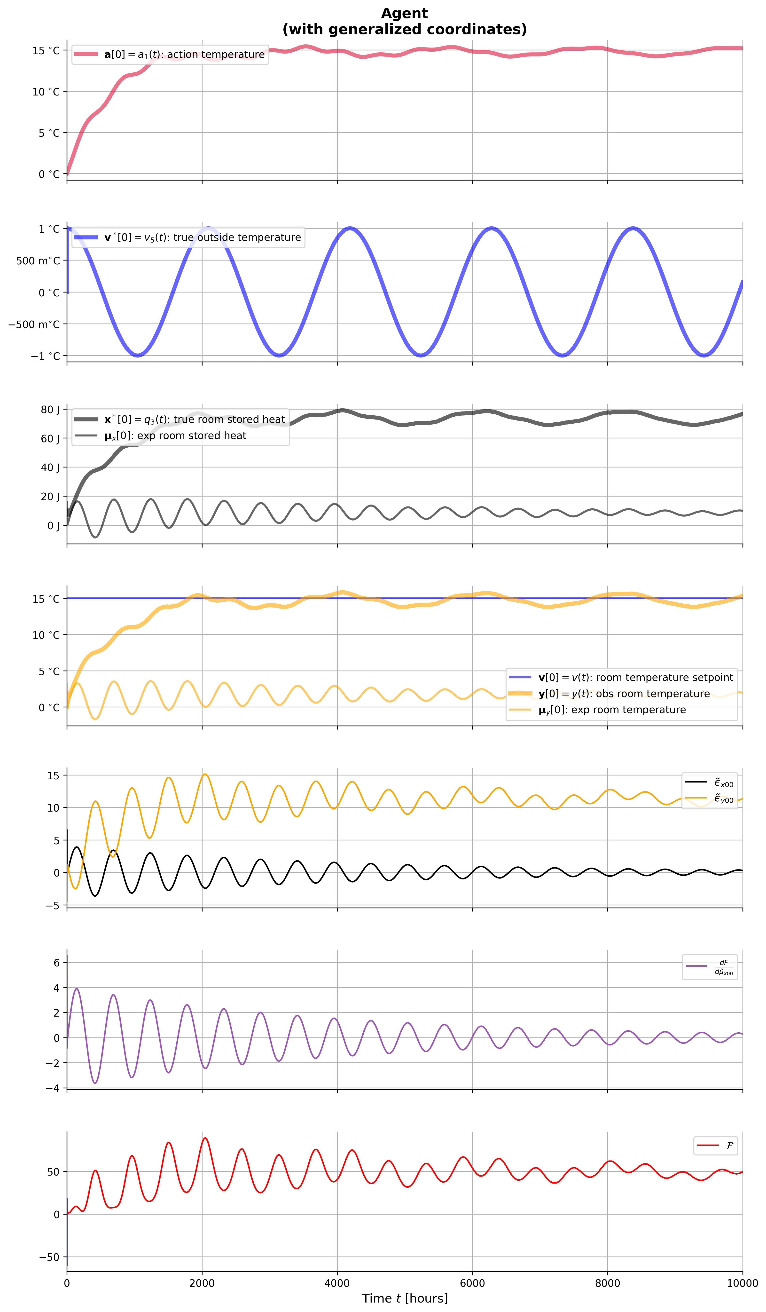
## plot_agent_result(result_agt)

from IPython.display import Image, display
display(Image(filename="ThermicSystem^v1-agent-withGC-step.png"))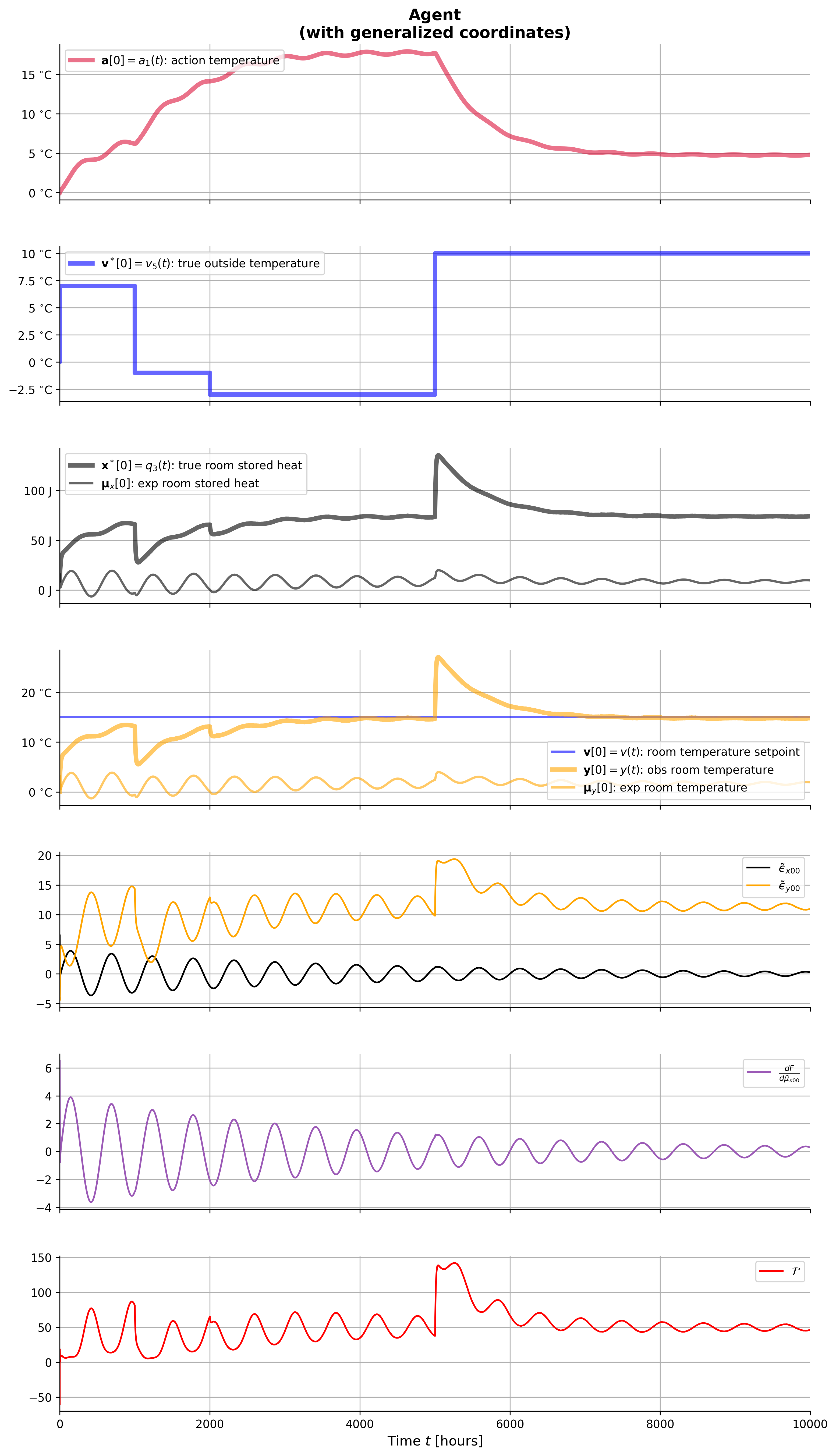

from IPython.display import Image, display
display(Image(filename="ThermicSystem^v1-agent-withGC-ramp.png"))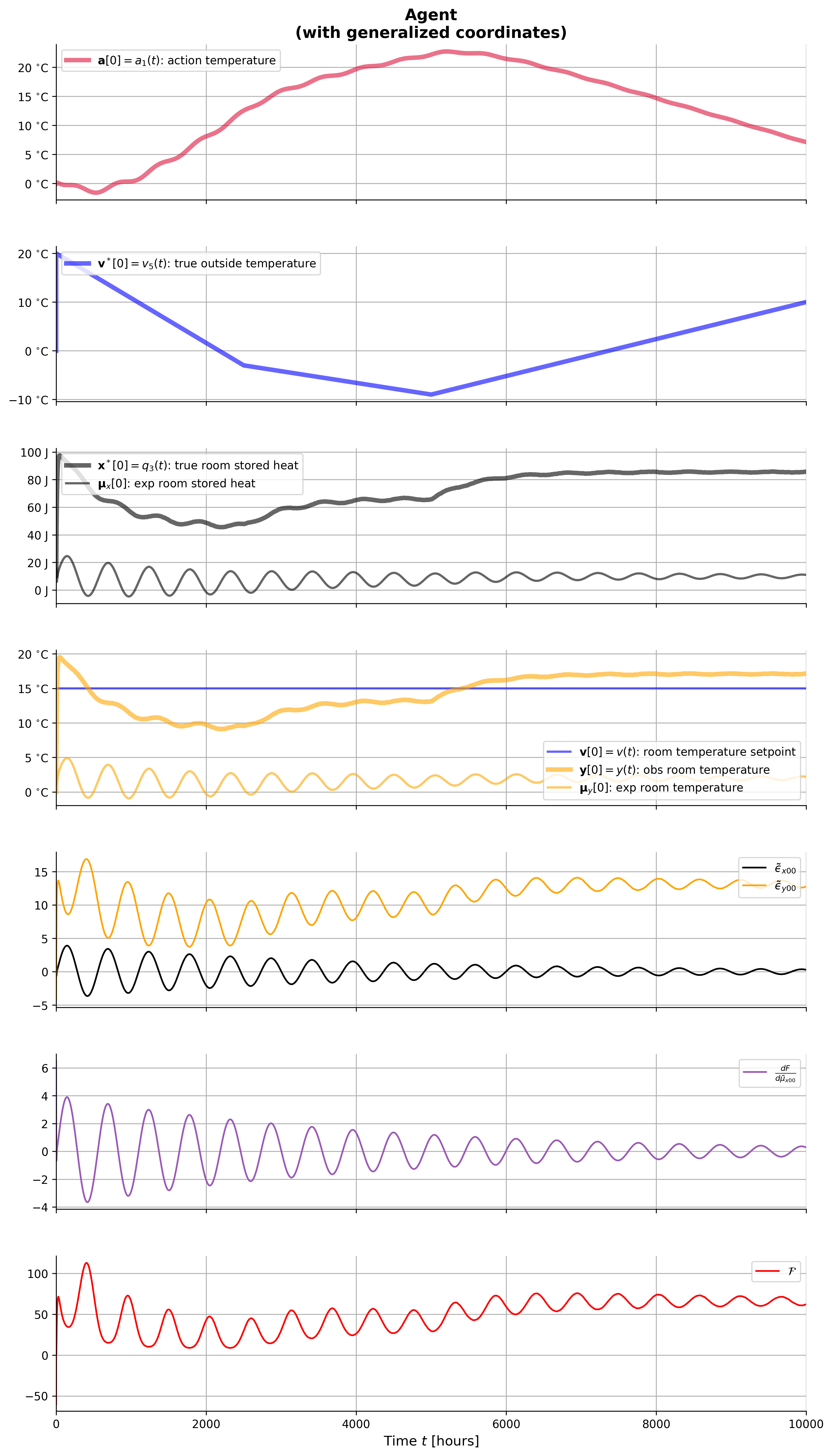

from IPython.display import Image, display
display(Image(filename="ThermicSystem^v1-agent-withGC-cos.png"))