T-maze Active Inference - Policy Inference (Part 1a)

Back to Portfolio of Projects |  LearnableLoopAI.com |  Blog | 

The overall purpose of the project is to lay the ground work for another project that makes use of a categorical control space. The purpose of the Part 1a project is to work through the following paper to gain a thorough understanding of its contents:

Koudahl, M. T., van de Laar, T. W., & de Vries, B. (2023). Realising Synthetic Active Inference Agents, Part I: Epistemic Objectives and Graphical Specification Language arXiv:2306.08014

It is not usually possible to make effective analysis annotations and expansions inside a pdf document. This notebook attempts to provide a remedy. Its contents is in the form of:

• Reproducing most of the content of the paper
• Structuring parts of the content
• Adding annotations, comments, and emphases
• Expanding mathematical expressions
• Rearranging mathematical expressions
• Changing mathematical symbols to align with my preferences

My additions are usually included within {{my addition}} or [[my addition]]. If in doubt about any part of the content of this notebook, please consult the original paper.

T-maze Active Inference - Policy Inference (Part 1a)

Abstract

The Free Energy Principle (FEP) is a theoretical framework for describing how (intelligent) systems self-organise into coherent, stable structures by minimising a free energy functional. Active Inference (AIF) is a corollary of the FEP that specifically details how systems that are able to plan for the future (agents) function by minimising particular free energy functionals that incorporate information seeking components. This paper is the first in a series of two where we derive a synthetic version of AIF on free form factor graphs. The present paper focuses on deriving a local version of the free energy functionals used for AIF. This enables us to construct a version of AIF which applies to arbitrary graphical models and interfaces with prior work on message passing (MP) algorithms. The resulting messages are derived in our companion paper. We also identify a gap in the graphical notation used for factor graphs. While factor graphs are great at expressing a generative model, they have so far been unable to specify the full optimisation problem including constraints. To solve this problem we develop constrained Forney-style factor graph (CFFG) notation which permits a fully graphical description of variational inference objectives. We then proceed to show how CFFGs can be used to reconstruct prior algorithms for AIF as well as derive new ones. The latter is demonstrated by deriving an algorithm that permits direct policy inference for AIF agents, circumventing a long standing scaling issue that has so far hindered the application of AIF in industrial settings. We demonstrate our algorithm on the classic T-maze task and show that it reproduces the information seeking behaviour that is a hallmark feature of AIF.

1 Introduction

Active Inference (AIF) is an emerging framework for modelling intelligent agents interacting with an environment. Originating in the field of computational neuroscience, it has since been spread to numerous other fields such as modern machine learning. At its core, AIF relies on variational inference techniques to minimise a free energy functional. A key differentiator of AIF compared to other approaches is the use of custom free energy functionals such as Expected and Generalised free energies (expected free energy (EFE) and generalised free energy (GFE), respectively). These functionals are specifically constructed so as to elicit epistemic, information-seeking behaviour when used to infer actions.

Optimisation of these functionals have so far relied on custom algorithms that require evaluating very large search trees which has rendered upscaling of AIF difficult. Many recent works, such as Branching Time AIF [3] and sophisticated inference [7] have investigated algorithmic ways to prune the search tree in order to solve this problem.

This paper is the first in a series of two parts where we take a different approach and formulate a variation of the GFE optimisation problem using a custom Lagrangian derived from constrained Bethe free energy (CBFE) on factor graphs. Using variational calculus we then derive a custom MP algorithm that can directly solve for fixed points of local GFE terms, removing the need for a search tree. This allows us to construct a purely optimisation-based approach to AIF which we name Lagrangian Active Inference (LAIF).

LAIF applies to arbitrary graph topologies and interfaces with generic MP algorithms which allow for scaling up of AIF using off-the-shelf tools. We accomplish this by constructing a node-local GFE on generic factor graphs.

The present paper is structured as follows: In section 2, we review relevant background material concerning Forney-style factor graphs (FFGs) and Bethe free energy (BFE). In section 3 we formalise what we mean by “epistemics” and construct an objective that is local to a single node on an FFG and possesses an epistemic, information-seeking drive. This objective turns out to be a local version of the GFE which we review in section 3.2.

Once we start modifying the free energy functional, we recognise a problem with current FFG notation. FFGs visualise generative models but fail to display a significant part of the optimisation problem, namely, the variational distribution and the functional to be optimised.

To remedy this, we develop the CFFG graphical notation in section 5 as a method for visualising both the variational distribution and any adaptations to the free energy functional that are needed for AIF. These tools form the basis of the update rules derived in our companion paper [15].

With the CFFG notation in hand, in section 6 we then proceed to demonstrate how to recover prior algorithms for AIF as MP on a CFFG. AIF is often described as MP on a probabilistic graphical model, see [4, 6, 13, 26] for examples. However, this relationship has not been properly formalised before, in part because adequate notation has been lacking. Using CFFGs it is straightforward to accurately write down this relation. Further, due to the modular nature of CFFGs it becomes easy to devise extensions to prior AIF algorithms that can be implemented using off-the-shelf MP tools.

Finally, section 7 demonstrates a new algorithm for policy inference using LAIF that scales linearly in the planning horizon, providing a solution to a longstanding barrier for scaling AIF to larger models and more complex tasks.

2 The Lagrangian approach to message passing

In this section, we review the Bethe free energy along with FFGs. These concepts form the foundation from which we will build towards local epistemic, objectives.

As a free energy functional, the BFE is unique because stationary points of the BFE correspond to solutions of the belief propagation algorithm [20, 25, 28] which provides exact inference on tree-structured graphs.

Furthermore, by adding constraints to the BFE using Lagrange multipliers, one can form a custom Lagrangian for an inference problem. Taking the first variation of this Lagrangian, one can then solve for stationary points and obtain MP algorithms that solve the desired problem. Prior work [25, 28] have shown that adding additional constraints to the BFE allows for deriving a host of different message passing algorithms including variational message passing (VMP) [27] and expectation propagation (EP) [18] among others. We refer interested readers to [25] for a comprehensive overview of this technique and how different choices of constraints can lead to different algorithms.

Constraints are specified at the level of nodes and edges, meaning this procedure can produce hybrid MP algorithms, foreshadowing the approach we are going to take for deriving a local, epistemic objective for AIF.

2.1 Bethe free energy and Forney-style factor graphs

Throughout the remainder of the paper we will use FFGs to visualise probabilistic models. In Section 5 we extend this notation to additionally allow for specifying constraints on the variational optimisation objective.

Following [25] we

• define an FFG as a graph $\mathcal{G}=(\mathcal{N},\mathcal{E})$ with
  • nodes $\mathcal{N}$ and
  • edges $\mathcal{E}\subseteq \mathcal{N}\times \mathcal{N}$.

For a node $a\in \mathcal{N}$ we denote the connected edges by $\mathcal{E}(a)$.

For an edge $i\in \mathcal{E}$, we denote the connected nodes by $\mathcal{N}(i)$.

An FFG can be used to represent a factorised function (model) over variables $\mathit{v}$, as [[‘a’ represents a node which is also square]]

$$f(\mathit{v})=\prod _{a\in \mathcal{N}}{f}_a({\mathit{v}}_a)$$

where ${\mathit{v}}_a$ collects the argument variables of the factor $f_a$. Throughout this paper we will use $\mathit{c}\mathit{u}\mathit{r}\mathit{s}\mathit{i}\mathit{v}\mathit{e}\mathit{b}\mathit{o}\mathit{l}\mathit{d}$ font to denote collections of variables. In the corresponding FFG, the factor $f_a$ is denoted by a square node and connected edges $\mathcal{E}(a)$ represent the argument variables ${\mathit{v}}_a$.

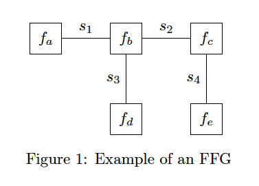
As an example, we can consider the FFG shown in Fig. 1

{{We replace ${\mathit{s}}_{\mathit{i}}$ with ${\mathit{v}}_{\mathit{i}}$. Later, we use $s_t$ for agent states and do not want to cause confusion. Here we use $v$ for a generic variable.}}:

Fig 1

{{

NOTE ON TERMINOLOGY

• joint, marginal, conditional are contractions for joint distribution, marginal distribution, and conditional distribution
• joint, marginal, conditional are relative terms
  • marginal refers to ‘summed/integrated-out’ factors relative to a starting joint
  • conditional refers to ‘conditioned-out’ factors relative to a starting joint
• example 1

For the model in Figure 1, we have that $$\underset{\begin{array}{c}\text{model}\\ \text{joint}\end{array}}{\underbrace{f(v_1,v_2,v_3,v_4)}}=\underset{\begin{array}{c}\text{model}\\ \text{marginal}\end{array}}{\underbrace{f_a(v_1)}}\underset{\begin{array}{c}\text{model}\\ \text{marginal}\end{array}}{\underbrace{f_b(v_1,v_2,v_3)}}\underset{\begin{array}{c}\text{model}\\ \text{marginal}\end{array}}{\underbrace{f_c(v_2,v_4)}}\underset{\begin{array}{c}\text{model}\\ \text{marginal}\end{array}}{\underbrace{f_d(v_3)}}\underset{\begin{array}{c}\text{model}\\ \text{marginal}\end{array}}{\underbrace{f_e(v_4)}}$$

• example 2

Assuming the model in Figure 1, were factored as follows: $$\underset{\begin{array}{c}\text{model}\\ \text{joint}\end{array}}{\underbrace{f(v_1,v_2,v_3,v_4)}}=\underset{\begin{array}{c}\text{model}\\ \text{marginal}\end{array}}{\underbrace{f_a(v_1,v_2)}}\underset{\begin{array}{c}\text{model}\\ \text{conditional}\end{array}}{\underbrace{f_b(v_3\mid v_4)}}\underset{\begin{array}{c}\text{model}\\ \text{marginal}\end{array}}{\underbrace{f_c(v_4)}}$$

• example 3

Let us focus in on the node factor $f_a(v_1,v_2)$. This factor is now the joint relative to which marginals/conditionals are referred to. Let us assume this joint factorizes as follows: $$\underset{\begin{array}{c}\text{node}\\ \text{joint}\end{array}}{\underbrace{f_a(v_1,v_2)}}=\underset{\begin{array}{c}\text{node}\\ \text{conditional}\end{array}}{\underbrace{f(v_1\mid v_2)}}\underset{\begin{array}{c}\text{node}\\ \text{marginal}\end{array}}{\underbrace{f(v_2)}}$$

}}

Fig 1 corresponds to the model

$$\begin{array}{}\text{(2)}& f(v_1,v_2,v_3,v_4)=f_a(v_1)f_b(v_1,v_2,v_3)f_c(v_2,v_4)f_d(v_3)f_e(v_4)\end{array}$$

In Fig. 1, the node set is $\mathcal{N}=\{a,...,e\}$ and the edge set is $\mathcal{E}=\{1,...,4\}$. As an example, the neighbouring edges of the node $c$ are given by $\mathcal{E}(c)=\{2,4\}$. In this way, FFGs allow for a simple visualisation of the factorisation properties of a high-dimensional function.

The problem we will focus on concerns minimisation of a {{variational}} free energy functional over a generative model. More formally, given a model (1) and a “variational” distribution $q(\mathit{v})$, the variational free energy (VFE) is defined as

$$\begin{array}{rl}F[q]& :={\mathbb{E}}_q\left[\text{log}\frac{q(\mathit{v})}{f(\mathit{v})}\right]\\ & =\int \text{log}\frac{q(\mathit{v})}{f(\mathit{v})}q(\mathit{v})\text{d}\mathit{v}\end{array}$$

The ‘[]’ means the argument is a function.

Variational inference concerns minimising this functional, leading to the solution:

$$\begin{array}{}\text{(4)}& q^{\ast }=\arg \underset{q\in \mathcal{Q}}{min}F[q]\end{array}$$

with $\mathcal{Q}$ denoting the admissible family of functions $q$. The optimised VFE upper-bounds the negative log-evidence (surprisal), as

$$\begin{array}{}\text{(5)}& f[q^{\ast }]=\underset{\text{Posterior divergence}}{\underbrace{\int \text{log}\frac{q^{\ast }(\mathit{v})}{p(\mathit{v})}{q}^{\ast }(\mathit{v})\text{d}\mathit{v}}}\underset{\text{Surprisal}}{\underbrace{-\text{log}Z}}\end{array}$$ where

• $Z=\int f(\mathit{v})\text{d}\mathit{v}$ is the model evidence
• $p(\mathit{v})=f(\mathit{v})/Z$ is the exact posterior

The BFE applies the Bethe assumption to the factorisation of $q$ which yields an objective that decomposes into a sum of local free energy terms, each local to a node on the corresponding FFG. Each node local free energy will include entropy terms from all connected edges. Since an edge is connected to (at most) two nodes, that means the corresponding entropy term would be counted twice. To prevent overcounting of the edge entropies, the BFE includes additional entropy terms that cancel out overcounted terms.

Under the Bethe approximation $q(\mathit{v})$ is given by

$$\begin{array}{}\text{(6)}& q(\mathit{v})=\prod _{a\in \mathcal{N}}{q}_a({\mathit{v}}_a)\prod _{i\in \mathcal{E}}{q}_i({\mathit{v}}_i{)}^{1-d_i}\end{array}$$ where $d_i$ is the degree of edge $i$. {{ $d_i\in \{1,2\}$ }}

As an example, on the FFG shown in Fig. 1 this would correspond to a variational distribution of the form

$$\begin{array}{}\text{(7)}& q(v_1,v_2,v_3,v_4)=\frac{q_a(v_1)q_b(v_1,v_2,v_3)q_c(v_2,v_4)q_d(v_3)q_e(v_4)}{q_1(v_1)q_2(v_2)q_3(v_3)q_4(v_4)}\end{array}$$ where we see terms for the

• ’n’odes in the ’n’umerator
• ’e’dges in the d’e’nominator

With this definition, the free energy factorises over the FFG as

$$\begin{array}{}\text{(8)}& \begin{array}{rl}F[q]& =\sum _{a\in \mathcal{N}}\underset{F[q_a]}{\underbrace{{\mathbb{E}}_{q_a}\left[\text{log}\frac{q_a({\mathit{v}}_a)}{f_a({\mathit{v}}_a)}\right]}}+\sum _{i\in \mathcal{E}}(1-d_i)\underset{H[q_i]}{\underbrace{{\mathbb{E}}_{q_i}\left[\text{log}\frac{1}{q_i({\mathit{v}}_i)}\right]}}\\ & =\sum _{a\in \mathcal{N}}\underset{F[q_a]}{\underbrace{\int \text{log}\frac{q_a({\mathit{v}}_a)}{f_a({\mathit{v}}_a)}{q}_a({\mathit{v}}_a)\text{d}{\mathit{v}}_a}}+\sum _{i\in \mathcal{E}}(1-d_i)\underset{H[q_i]}{\underbrace{\int \text{log}\frac{1}{q_i({\mathit{v}}_i)}{q}_i({\mathit{v}}_i)\text{d}{\mathit{v}}_i}}\end{array}\end{array}$$

Eq. (8) defines the BFE. Note that $F$ defines a free energy functional which can be either local or global depending on its arguments. More specifically,

• $F[q]$ defines the free energy for the entire model, while
• $F[q_a]$ defines a node-local (to the node $a$) BFE contribution of the same functional form.

Under optimisation of the BFE, i.e. solving Eq. (4), $q^{\ast }=\arg \underset{q\in \mathcal{Q}}{min}F[q]$, the admissible set of functions $\mathcal{Q}$ enforces consistent normalisation and marginalisation of the node and edge local distributions, such that

$$\begin{array}{}\text{(9a)}& \int q_i({\mathit{v}}_i)\text{d}{\mathit{v}}_i=1\text{for all}i\in \mathcal{E}\end{array}$$ $$\begin{array}{}\text{(9b)}& \int q_a({\mathit{v}}_a)\text{d}{\mathit{v}}_a=1\text{for all}a\in \mathcal{N}\end{array}$$ $$\begin{array}{}\text{(9c)}& \int q_a({\mathit{v}}_a)\text{d}{\mathit{v}}_{a\mathrm{\setminus }i}=q_i({\mathit{v}}_i)\text{for all}a\in \mathcal{N},i\in \mathcal{E}(a)\end{array}$$

Because we always assume the constraints given by Eq. (9) to be in effect, we will omit the subscript on individual q’s moving forwards and instead let the arguments determine which marginal we are referring to, for example writing $q(v_a)$ instead of $q_a(v_a)$.

A core aspect of FFGs is that they allow for easy visualisation of MP algorithms. MP algorithms are a family of distributed inference algorithms with the common trait that they can be viewed as messages flowing on an FFG.

As a general rule, to infer a marginal for a variable,

• messages are passed on the graph toward the associated edge for that variable
• multiplication of colliding (forward and backward) messages on an edge yields the desired posterior marginal

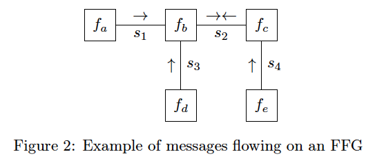
We denote a message on an FFG by arrows pointing in the direction that the message flows.

We show an example in Fig. 2 of inferring a posterior marginal for the variable $v_2$. In this example, messages are flowing on the FFG of Fig. (1) towards the variable $v_2$ where we see two arrows colliding. The exact form of the individual messages depend on the algorithm being used.

Fig2

3 Defining epistemic objectives

Now we move on to the central topic of AIF, namely agents that interact with the world they inhabit.

Under the heading of AIF, an agent

• entails a generative model of its environment, and
• is engaged in the process of achieving future goals (specified by a target distribution or goal prior) through actions.
• This task can be cast as a process of free energy minimisation [5, 7, 8].

A natural question to ask is then, what should this free energy functional look like and why? Here we wish to highlight a

• core feature of AIF that sets it apart from other approaches:
  • Systematic information gathering by targeted exploration of an environment.

Whatever the form of our free energy functional, it should lead to agents that possess an exploratory drive consistent with AIF.

While it is tempting to default to a standard VFE, prior work [24] has shown that directly optimising BFE or VFE when inferring a sequence of actions (which we will refer to as a policy) does not lead to agents that systematically explore their environment. Instead,

• directly inferring a policy by minimising a VFE/BFE leads to Kullback-Leibler divergence (KL)-control [12] 1.

This means that VFE/BFE is not the correct choice when we desire an agent that actively samples its environment with the explicit purpose of gathering information.

Instead a hallmark feature of AIF is the use of alternative functionals in place of either the VFE or the BFE, specifically for inferring policies. The goal of these alternative functionals is often specifically to induce an epistemic, explorative term that drives AIF agents to seek out information.

Epistemics, epistemic behaviour or “foraging for information” are commonly used terms in the AIF literature and related fields. While we have used the term colloquially until this point, we now clarify formally how we use the term in the present paper and how it relates to the objective functionals we consider. A core problem is that epistemics is most often defined in terms of the behaviour of agents (“what does my agent do?”) rather than from a mathematical point of view. Prior work on this point includes [10, 17].

We take the view that epistemics arise from the optimisation of either an mutual information (MI) {{aka Information Gain}} term or a bound thereon. The MI (between two variables $x$ and $s$) is defined as [16]

{{‘Expectation-log of the joint over the marginals’}}

$$\begin{array}{}\text{(10)}& \begin{array}{rl}\text{I}[x,s]& ={\mathbb{E}}_p\left[\log \frac{p(x,s)}{p(x)p(s)}\right]\\ & =\int \int \log \frac{p(x,s)}{p(x)p(s)}p(x,s)\mathrm{d}x\mathrm{d}s\end{array}\end{array}$$

To gain an intuition for why maximising MI leads to agents that seek out information, we can rewrite MI {{i.e. (10)}} as

$$\begin{array}{}\text{(11)}& \begin{array}{rl}\text{I}[x,s]& ={\mathbb{E}}_p\left[\log \frac{p(x,s)}{p(x)p(s)}\right]\\ & =\int \int \log \frac{p(x,s)}{p(x)p(s)}p(x,s)\mathrm{d}x\mathrm{d}s\\ & =\int \int \log \frac{\stackrel{\text{flipped}x,s}{\overbrace{p(s,x)}}}{p(x)p(s)}p(x,s)\mathrm{d}x\mathrm{d}s\\ & =\int \int \log \frac{p(s\mid x)p(x)}{p(x)p(s)}p(x,s)\mathrm{d}x\mathrm{d}s\\ & =\int \int \log \frac{p(s\mid x)}{p(s)}p(x,s)\mathrm{d}x\mathrm{d}s\text{(cancelation)}\\ & =\mathrm{H}[s]-\mathrm{H}[s\mid x]=\mathrm{H}[x]-\mathrm{H}[x\mid s]\end{array}\end{array}$$

Since MI is symmetric in its arguments, Eq. (11) can equally well be written in terms of $x$ rather than $s$. Eq. (11) shows that MI decomposes as the difference between the marginal entropy $s$ and the expected entropy of $s$ conditional on $x$.

If we let

• $s$ denote an internal state of an agent and
• $x$ an observation and
• allow our agent to choose $x$ (for instance through acting on an environment)

we can see why maximising Eq. (10) biases the agent towards seeking our observations that reduce entropy in $s$. Maximising Eq. (10) means the agent will prefer observations that provide useful (in the sense of reducing uncertainty) information about its internal states $s$. For this reason MI is also known as Information Gain.

Actually computing Eq. (10) is often intractable and in practice, a bound is often optimised instead.

3.1 Constructing a local epistemic objective

At this point, we have seen that the BFE

• is distributed over arbitrary FFGs
• does not lead to epistemic behaviour

On the other hand, maximising MI

• is not distributed over arbitrary FFGs
• leads to the types of epistemic behaviour we desire

The question becomes whether there is a way to merge the two and obtain a distributed functional - like the BFE - that includes an epistemic term?

We will now show how to construct such a functional. Our starting point will be the BFE given by Eq. (8), {{repeated here:}} $$\begin{array}{}\text{(8)}& \begin{array}{rl}F[q]& =\sum _{a\in \mathcal{N}}\underset{F[q_a]}{\underbrace{{\mathbb{E}}_{q_a}\left[\text{log}\frac{q_a({\mathit{v}}_a)}{f_a({\mathit{v}}_a)}\right]}}+\sum _{i\in \mathcal{E}}(1-d_i)\underset{H[q_i]}{\underbrace{{\mathbb{E}}_{q_i}\left[\text{log}\frac{1}{q_i({\mathit{v}}_i)}\right]}}\\ & =\sum _{a\in \mathcal{N}}\underset{F[q_a]}{\underbrace{\int \text{log}\frac{q_a({\mathit{v}}_a)}{f_a({\mathit{v}}_a)}{q}_a({\mathit{v}}_a)\text{d}{\mathit{v}}_a}}+\sum _{i\in \mathcal{E}}(1-d_i)\underset{H[q_i]}{\underbrace{\int \text{log}\frac{1}{q_i({\mathit{v}}_i)}{q}_i({\mathit{v}}_i)\text{d}{\mathit{v}}_i}}\end{array}\end{array}$$

We will focus on a single node $a$ and its associated local energy term and partition the incoming edges into two sets, $\mathit{x}$ and $\mathit{s}$.

This gives the node local {{variational}} free energy

$$\begin{array}{}\text{(12)}& \begin{array}{rl}F[q_a]& ={\mathbb{E}}_{q_a}\left[\text{log}\frac{q(\mathit{x},\mathit{s})}{f(\mathit{x},\mathit{s})}\right]\\ & =\int \int \log \frac{q(\mathit{x},\mathit{s})}{f(\mathit{x},\mathit{s})}q(\mathit{x},\mathit{s})\mathrm{d}\mathit{x}\mathrm{d}\mathit{s}\end{array}\end{array}$$

Now we need to add on an MI {{aka IG}} term to induce epistemics. Since we are

• minimising our free energy functional and want to
• maximise MI,

we augment the free energy with a negative MI term as

$$ $$\begin{array}{}\text{(13)}& \begin{array}{rl}\mathcal{G}[q_a]& =\stackrel{\text{Variational free energy}}{\overbrace{{\mathbb{E}}_{q_a}\left[\text{log}\frac{q(\mathit{x},\mathit{s})}{f(\mathit{x},\mathit{s})}\right]}}+\stackrel{\text{Negative mutual information}}{\overbrace{{\mathbb{E}}_{q_a}\left[\text{log}\frac{q(\mathit{x})q(\mathit{s})}{q(\mathit{x},\mathit{s})}\right]}}(13a)\\ & ={\mathbb{E}}_{q_a}[\text{log}\frac{q(\mathit{x},\mathit{s})}{f(\mathit{x},\mathit{s})}+\text{log}\frac{q(\mathit{x})q(\mathit{s})}{q(\mathit{x},\mathit{s})}]\\ & ={\mathbb{E}}_{q_a}[\text{log}q(\mathit{x},\mathit{s})-\text{log}f(\mathit{x},\mathit{s})+\text{log}q(\mathit{x})q(\mathit{s})-\text{log}q(\mathit{x},\mathit{s})]\\ & ={\mathbb{E}}_{q_a}[\text{log}q(\mathit{x})q(\mathit{s})-\text{log}f(\mathit{x},\mathit{s})](13b)\\ & ={\mathbb{E}}_{q_a}\left[\text{log}\frac{q(\mathit{x})q(\mathit{s})}{f(\mathit{x},\mathit{s})}\right](13c)\\ & =\int \int \text{log}\frac{q(\mathit{x})q(\mathit{s})}{f(\mathit{x},\mathit{s})}q(\mathit{x},\mathit{s})\mathrm{d}\mathit{x}\mathrm{d}\mathit{s}\end{array}\end{array}$$

$$

which we can recognise as a node-local GFE [19]. In section 3.2 we review the results of [19] to expand upon this statement. Eq. (13a) provides a straightforward explanation of the kinds of behaviour that we can expect out of agents optimising a GFE. Namely, minimising BFE with a goal prior corresponds to performing KL-control [12] while the MI term adds an epistemic, information-seeking component. Viewed in this way, there is nothing mysterious about the kind of objective optimised by AIF agents: It is simply the sum of two wellknown and established objectives that are each widely used within the control and reinforcement learning communities.

3.2 Generalized free energy

The objective derived in Eq. (13) is a node local version of the GFE originally introduced by [19]. In this section, we review the GFE as constructed by [19] in order to relate our construction to prior work on designing AIF functionals. In section 6, we show how to reconstruct the exact method of [19] using the tools we develop in this paper. Prior to [19], the functional of choice was the EFE [4, 6]. [19] identified some issues with the EFE and proposed the GFE as a possible solution.

We show how to reconstruct the original EFE-based algorithm of [6] using our local objective in section 6. We also provide a detailed description of the EFE in Appendix. A since it is still a popular choice for designing AIF agents.

A core issue with the EFE is that it is strictly limited to planning over future timesteps. This means that

• AIF agents that utilise the EFE functional need to maintain two separate models:
  • One for inferring policies (using EFE) and
  • one for state inference (using VFE/BFE) that updates as observations become available.

The key advantage of EFE is that it induces the epistemic drive that we desire from AIF agents.

The goal of [19] was to extend upon the EFE by introducing a functional that could induce similar epistemic behaviour when used to infer policies while at the same time reducing to a VFE when dealing with past data points. In this way, an agent would no longer have to maintain two separate models and could instead utilise only one.

The GFE as introduced by [19] is tied to a specific choice of generative model. The model introduced by [19] is given by

$$\begin{array}{}\text{(14)}& \begin{array}{rl}p(\mathbf{x},\mathbf{s}\mid \hat{\mathbf{u}})& \propto \underset{\begin{array}{c}\text{Initial}\\ \text{state}\\ \text{prior}\end{array}}{\underbrace{p({\mathbf{s}}_0)}}\prod _{k=1}^T\underset{\begin{array}{c}\text{Observation}\\ \text{model}\end{array}}{\underbrace{p({\mathbf{x}}_k\mid {\mathbf{s}}_k)}}\underset{\begin{array}{c}\text{Transition}\\ \text{model}\end{array}}{\underbrace{p({\mathbf{s}}_k\mid {\mathbf{s}}_{k-1},{\hat{\mathbf{u}}}_k}})\underset{\begin{array}{c}\text{Goal}\\ \text{prior}\end{array}}{\underbrace{p^{+}({\mathbf{x}}_k)}}\end{array}\end{array}$$

where

• $\mathbf{x}$ denotes observations
• $\mathbf{s}$ denotes latent states
• $\hat{\mathbf{u}}$ denotes a fixed policy

Throughout this paper we will use $t$ to refer to the current time step in a given model and denote fixed values by a hat, here exemplified by $\hat{\mathbf{u}}$. Further, we also use $\mathbf{s}$ to denote {{1-hot ?}} vectors.

Given a current time step $t$, we have that for future time steps $k>t$, $p^{+}({\mathbf{x}}_k)$ defines a goal prior over desired future observations. For past time steps $k\le t$, we instead have $p^{+}({\mathbf{x}}_k)=1$ which makes it uninformative 2. Writing the model in this way allows for a single model for both

• perception (integrating past data points) and
• action (inferring policies)

since both past and future time steps are included. GFE is defined as [19]

$$\begin{array}{}\text{(15)}& \begin{array}{rl}\mathcal{G}[q;\hat{\mathbf{u}}]& =\sum _{k=1}^T{\mathbb{E}}_q\left[\text{log}\frac{q({\mathbf{x}}_k\mid {\hat{\mathbf{u}}}_k)q({\mathbf{s}}_k\mid {\hat{\mathbf{u}}}_k)}{p^{+}({\mathbf{x}}_k),p({\mathbf{x}}_k,{\mathbf{s}}_k\mid {\hat{\mathbf{u}}}_k)}\right]\\ & =\sum _{k=1}^T\int \int \left[\text{log}\frac{q({\mathbf{x}}_k\mid {\hat{\mathbf{u}}}_k)q({\mathbf{s}}_k\mid {\hat{\mathbf{u}}}_k)}{p^{+}({\mathbf{x}}_k),p({\mathbf{x}}_k,{\mathbf{s}}_k\mid {\hat{\mathbf{u}}}_k)}\right]q({\mathbf{x}}_k\mid {\mathbf{s}}_k)q({\mathbf{s}}_k\mid {\hat{\mathbf{u}}}_k)\text{d}{\mathbf{x}}_k\text{d}{\mathbf{s}}_k\end{array}\end{array}$$

where

$$q({\mathbf{x}}_k,{\mathbf{s}}_k)=\{\begin{array}{ll}\delta ({\mathbf{x}}_k-{\hat{\mathbf{x}}}_k)& \text{if }k\le t\\ p({\mathbf{x}}_k\mid {\mathbf{s}}_k)& \text{if }k>t\end{array}$$

and ${\hat{\mathbf{x}}}_k$ denotes the observed data point at time step $k$. $p({\mathbf{x}}_k,{\mathbf{s}}_k\mid {\hat{\mathbf{u}}}_k)$ can be found recursively by Bayesian smoothing, see [14, 23] for details. To see how the GFE reduces to a VFE when data is available, we refer to Appendix B.

The GFE introduced by [19] improves upon prior work utilising EFE but still has some issues. The first lies in tying it to the model efinition in Eq. (14). Being committed to a model specification apriori severely limits what the GFE can be applied to since not all problems are going to fit the model specification. Additionally, a more subtle issue lies in the commitment to a hard time horizon. If t denotes the current timestep, at some point time will advance to the point $t>T$. When this happens Eq. (14) loses the capacity to plan and becomes static since all observations are clamped by Eq. (16). A further complication arises from $\hat{\mathbf{u}}$ being a fixed parameter and not a random variable. Being a fixed parameter means it is not possible to perform inference for $\hat{\mathbf{u}}$ which in turn makes scaling difficult. Moving to a fully local version of the GFE instead means we can construct a new synthetic approach to AIF that addresses these issues.

4 LAIF - Lagrangian Active Inference

Armed with the node local GFE derived in Eq. (13), we can construct a Lagrangian for AIF. The goal is to adapt the Lagrangian approach to MP sketched in section 2 to derive a MP algorithm that optimises local GFE in order to have a distributed inference procedure that incorporates epistemic terms. Naively applying the method of [25] to Eq. (13) does not yield useful results because the numerator differs from the term we take the expectation with respect to. To obtain a useful solution we need that

$$q(\mathit{x}\mathbf{,}\mathit{s})=q(\mathit{x}\mid \mathit{s})q(\mathit{s})$$

and add the original assumption in [19], given by Eq. (16)

$$q(\mathit{x}\mid \mathit{s})\triangleq p(\mathit{x}\mid \mathit{s})$$

With these additional assumptions, we can obtain meaningful solutions and derive a message passing algorithm that optimises a local GFE and induces epistemic behaviour which we demonstrate in section7. The detailed derivation of these results can be found in our companion paper [15]. For practical AIF modelling, we provide the relevant messages in Fig. 21.

At this point, we will instead show a different way to arrive at the local GFE. This approach is more “mechanical” but has the advantage that it can more easily be written in terms of constraints on the BFE. Our starting point will once again be a free energy term local to the node $a$ {{‘Expectation-log of the q-joint over the f-joint’}}

$$\begin{array}{}\text{(19)}& \begin{array}{rl}F[q_a]& \triangleq {\mathbb{E}}_{q_a}\left[\text{log}\frac{q({\mathit{v}}_a)}{f({\mathit{v}}_a)}\right]\\ & =\int \text{log}\frac{q({\mathit{v}}_a)}{f({\mathit{v}}_a)}q({\mathit{v}}_a)\text{d}{\mathit{v}}_a\end{array}\end{array}$$

To turn Eq. (19) into a local** GFE we need to perform two steps.** - The first is to enforce a mean field factorisation

$$\begin{array}{}\text{(20)}& q({\mathit{v}}_a)=\prod _{i\in \mathcal{E}(a)}q(v_i)\end{array}$$

• The second is to change the expectation to obtain

$$\begin{array}{}\text{(21)}& \int \text{log}\frac{q({\mathit{v}}_a)}{f({\mathit{v}}_a)}\stackrel{\text{from}}{\overbrace{q({\mathit{v}}_a)}}\text{d}{\mathit{v}}_a⟹\int \text{log}\frac{q({\mathit{v}}_a)}{f({\mathit{v}}_a)}\stackrel{\text{to}}{\overbrace{p(v_i\mid {\mathit{v}}_{a\mathrm{\setminus }i})q({\mathit{v}}_{a\mathrm{\setminus }i})}}\text{d}{\mathit{v}}_a\end{array}$$

where $i\in \mathcal{E}(a)$. This partitions the connected variables into two sets:

• A set of variables where the expectation is modified and
• any remainder that is not modified.

$p(v_i\mid {\mathit{v}}_{a\mathrm{\setminus }i})$ denotes a conditional probability distribution. We write $p$ here instead of $f$ to emphasise that the conditional needs to be normalised in order for us to be able to take the expectation.

We refer to this move as a P-substitution. Once the mean field factorisation is enforced, we can recognise Eq. (21) as a node-local GFE $G[q_a]$.

As an example of constructing a node-local GFE with this approach, we can consider a node with two connected variables, $\{x,s\}$.

The local {{variational}} free energy becomes

$$\begin{array}{}\text{(22)}& \begin{array}{rl}F[q_a]& ={\mathbb{E}}_{q_a}\left[\text{log}\frac{q(x,s)}{p(x,s)}\right]\\ & =\int \int \log \frac{q(x,s)}{p(x,s)}q(x,s)\mathrm{d}x\mathrm{d}s\end{array}\end{array}$$

• Now we apply a mean field factorisation

$$\begin{array}{}\text{(23)}& \begin{array}{rl}F[q_a]& =\int \int \log \frac{q(x)q(s)}{p(x,s)}q(x)q(s)\mathrm{d}x\mathrm{d}s\end{array}\end{array}$$

• And finally, perform P-substitution to obtain a node-local GFE

$$\begin{array}{}\text{(24)}& \begin{array}{r}\int \int \log \frac{q(x)q(s)}{p(x,s)}\stackrel{\text{from}}{\overbrace{q(x)}}q(s)\mathrm{d}x\mathrm{d}s⟹\int \int \log \frac{q(x)q(s)}{p(x,s)}\stackrel{\text{to}}{\overbrace{p(x\mid s)}}q(s)\mathrm{d}x\mathrm{d}s\end{array}\end{array}$$

We denote the set of nodes for which we want to perform P-substitution with $\mathcal{P}\subseteq \mathcal{N}$.

When performing P-substitution, we are

• replacing a local variational free energy {{VFE}} $F[q_a]$
• with a local generalised free energy {{GFE}} $\mathcal{G}[q_a]$.

Armed with P-substitution, we can now write the simplest instance of a Lagrangian for Active Inference

$$\begin{array}{}\text{(25)}& \begin{array}{rl}\mathcal{L}[q]& =\underset{\begin{array}{c}\text{P-substituted}\\ \text{subgraph with}\\ \text{naive mean field}\end{array}}{\underbrace{\sum _{a\in \mathcal{P}}\mathcal{G}[q_a]}}+\underset{\begin{array}{c}\text{Node local}\\ \text{free energies}\end{array}}{\underbrace{\sum _{b\in \mathcal{N}\mathrm{\setminus }\mathcal{P}}F[q_b]}}+\sum _{i\in \mathcal{E}}(1-d_i)\underset{\text{Edge entropy}}{\underbrace{\text{H}[q(v_i)]}}\\ & +\underset{\text{Marginalization}}{\underbrace{\sum _{a\in \mathcal{N}}\sum _{i\in \mathcal{E}}\int {\lambda }_{ia}(v_i)[q(v_i)-\int q({\mathit{v}}_a)\text{d}{v}_{a\mathrm{\setminus }i}]\text{d}{v}_i}}\\ & +\underset{\text{Normalization of node marginals}}{\underbrace{\sum _{a\in \mathcal{N}}{\lambda }_a[\int q({\mathit{v}}_a)\text{d}{v}_a-1]}}+\underset{\text{Normalisation of edge marginals}}{\underbrace{\sum _{i\in \mathcal{E}}{\lambda }_i[\int q(v_i)\text{d}{v}_i-1]}}\end{array}\end{array}$$

With the Active Inference Lagrangian in hand, we can now solve for stationary points using variational calculus and obtain MP algorithms for LAIF. The key insight is that messages flowing out of $\mathcal{P}$ derived from stationary points of Eq. (25) will correspond to stationary points of the local GFE rather than BFE, meaning the result will include an epistemic component. This paves the way for a localised version of AIF that applies to arbitrary graph structures, does not suffer from scaling issues as the planning horizon increases, and can be solved efficiently and asynchronously using MP.

5 Constrained Forney-style factor graphs

While FFGs are a useful tool for writing down generative models, we have by now established the importance of knowing the exact functional to be minimised. This requires specifying not just the model $f$ but also the family $\mathcal{Q}$ through constraints and any potential P-substitutions. This is important if we want to be able to succinctly specify not just the model but also the exact inference problem we aim to solve.

We will now develop just such a new notation for writing ::constraints:: directly as part of the FFG. We refer to ::FFGs with added constraints:: specification as CFFGs.

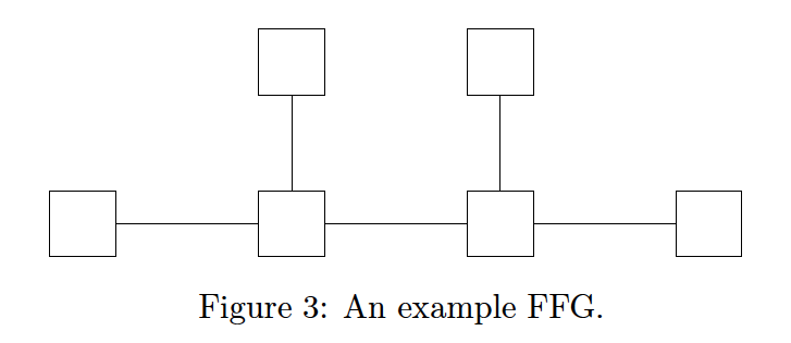
Fig 3 shows a model comprised of five edges and six nodes. FFGs traditionally represent the model $f$ using squares connected by lines as shown in Fig. 3. The squares represent factors and the connections between them represent variables. Connecting an edge to a square node indicates that the variable on that edge is an argument of the factor it is connected to.

The notation for CFFGs adheres to similar principles when specifying $f$. However, we

• augment the FFG with circular beads to
  • indicate the constraints that define our family $\mathcal{Q}$. Each factor of the variational distribution in $q$ will correspond to a bead and the
  • position of a bead indicates to which marginal it refers - a
    • bead on an edge denotes an
      • edge marginal $q(v_i)$ and a
    • bead inside a node denotes a
      • node marginal $q({\mathit{v}}_a)$.

An empty bead will denote the

• default normalisation constraints while a

connection between beads indicates

• marginalisation constraints following Eq. (9).

These beads form the basic building blocks of our notation.

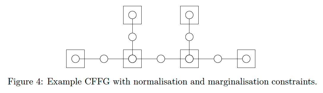
To write the objective corresponding to the model in Fig. 3 given the default constraints of Eq. (9), we add beads for every term and extend edges through the node boundary to connect variables that are under marginalisation constraints as shown in Fig. 4.

5.1 Factorisation constraints

We will now extend our notation with the most common types of constraints used for defining $\mathcal{Q}$. A common choice is factorisation of the variational distribution with the most well-known example being the naive mean field approximation. Under a naive mean-field factorisation, all marginals are considered independent. Formally this means we enforce

$$\begin{array}{}\text{(26)}& q({\mathit{v}}_a)=\prod _{i\in \mathcal{E}(a)}q(v_i)\end{array}$$

To write Eq. (26) on a CFFG we need to

• replace the joint node marginal
• with the product of adjacent edge marginals.

To do this we can

• replace the bead indicating the joint marginal
• with a bead for each edge marginal in Eq. (26) as shown in Fig. 5.

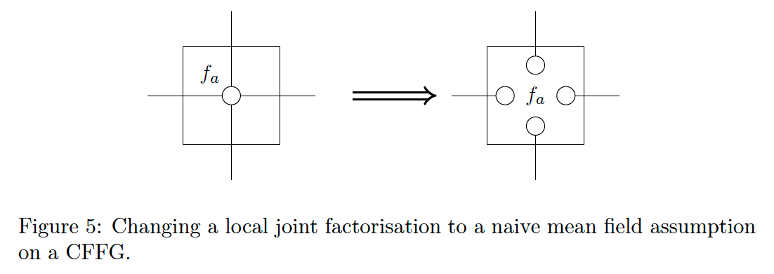
The strongest factorisation possible is the

• naive mean field factorization

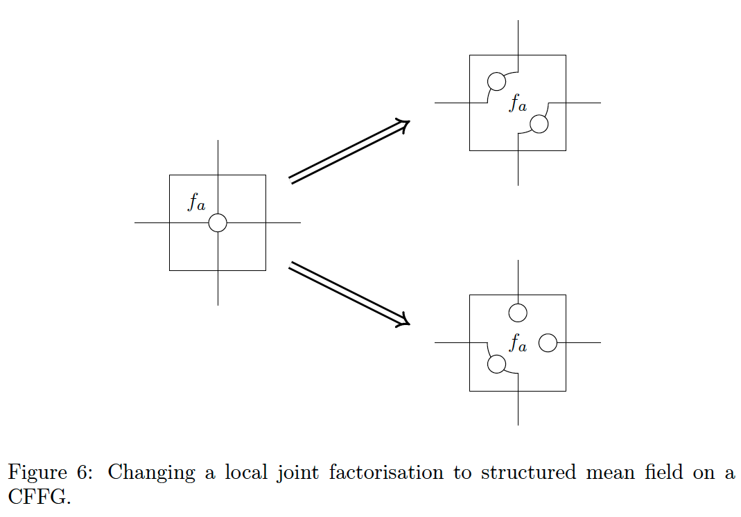
It is possible to utilise less aggressive factorisations by appealing to a

• structured mean field approximation instead.

The structured mean field constraint takes the form $$\begin{array}{}\text{(27)}& q({\mathit{v}}_a)=\prod _{n\in l(a)}{q}^n({\mathit{v}}_a^n)\end{array}$$ where $l(a)$ denotes a set of one or more edges connected to the node $a$ such that each element in $\mathcal{E}(a)$ can only appear in $l(a)$ once [25]. For example if $\mathcal{E}(a)=\{i,j,k\}$ corresponding to variables $\{x,y,z\}$, we can factorise $q(x,y,z)$ as $q(x)q(y,z)$ or $q(z)q(x,y)$ but not as $q(x,y)q(y,z)$ since $y$ appears twice. The naive mean field is a special case of the structured mean field where every variable appears only by itself.

To write a structured mean field factorisation on a CFFG we can apply a similar logic and replace the single bead denoting the joint with beads that match the structure of $l(a)$. Each set of variables that are factorised together corresponds to a single bead connected to the edges in the set that factor together.

Fig. 6 shows two example factorisations. The first option factorises the four incoming edges into two sets of two while the second partitions the incoming edges into two sets of one and a single set of two. Using these principles it is possible to specify complex factorisation constraints as part of the CFFG by augmenting each node on the original FFG.

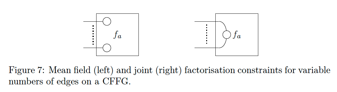
The final situation we need to consider is the case when a single node has a variable or very high number of incoming edges.

• An example could be a Gaussian Mixture Model with a variable number of mixture components.

On a CFFG we indicate variable or large numbers of identical edges by drawing two of the relevant edges and separating them with dots (· · · ) as shown in Fig. 7. To indicate factorisation constraints we can write either a joint or a naive mean field factorisation between the two edges, letting the dots denote that a similar factorisation applies to the remaining edges.

5.2 Form constraints

We will now extend CFFG notation with constraints on the functional form of nodes and edges. Form constraints are used to enforce a particular form for a local marginal on either an edge or a node.

• For an edge $v_i$ they enforce

$$\begin{array}{}\text{(28)}& \int q_a({\mathit{v}}_a)\text{d}{v}_{a\mathrm{\setminus }i}=q(v_i)=g(v_i)\end{array}$$

where $g(v_i)$ denotes the functional form we are constraining the edge marginal $v_i$ to take.

• Form constraints on node marginals take the form

$$\begin{array}{}\text{(29)}& q({\mathit{v}}_a)=g({\mathit{v}}_a)\end{array}$$

Conventionally FFGs denote the form of a factor by a symbol inside the node. We adopt a similar convention to denote form constraints on $q$ by adding symbols within the corresponding beads. For instance, we can indicate a Gaussian form constraint on an edge as shown in Fig 8

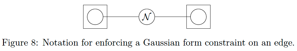
Note that this is not dependent on the form of the neighbouring factors. This is a subtle point as it allows us to write approximations into the specification of $\mathcal{Q}$. As an example, the unconstrained marginal in Fig 8 might be bimodal or highly skewed but by adding a form constraint, we are enforcing a Gaussian approximation. Outside of a few special cases, enforcing form constraints on edges is rarely done in practice since the functional form of $q$ most often follows from optimisation [25].

A special case of form constraints is the case of dangling edges (edges that are not terminated by a factor node). Technically these would not warrant a bead since they would not appear explicitly in the BFE due to having degree 1. Intuitively this means that the edge marginal is only counted once and we therefore do not need to correct for overcounting. However, without a bead, there is nowhere to annotate a form constraint which is problematic.

The solution for CFFG notation is to simply draw the bead anyway, in case a form constraint is needed. This is formally equivalent to terminating the dangling edge by a factor node with the node function $f_a({\mathit{v}}_a)=1$. Terminating the edge in this way means the edge in question now has degree 2 and therefore warrants a bead. This is always a valid move since multiplication by 1 does not change the underlying function [25].

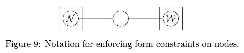
We can denote form constraints on node marginals in the same manner as edge marginals. We show an example in Fig 9 where we enforce a Gaussian form constraint on one node marginal and a Wishart on the other. Again it is important to note that these are constraints on $q$ and not part of the underlying model specification $f$.

Two kinds of form constraints warrant extra attention: $\delta$-constraints and moment matching. We will now deal with these in turn.

5.3 $\delta$-constraints and data points

$\delta$-constraints are the most commonly used form constraints because they allow us to incorporate data points into a model. A $\delta$-constraint on an edge defines the function $g(v_i)$ in Eq. (28) to be $$\begin{array}{}\text{(30)}& g(v_i)=\delta (v_i-{\hat{v}}_i)\end{array}$$

What makes the $\delta$-constraint special is that ${\hat{v}}_i$ can either be

• a known value or
• a parameter to optimise [25].

In the case where ${\hat{v}}_i$ is known,

• it commonly corresponds to a data point.
• We refer to this case as a data constraint and
• denote it with a filled circle as shown in Fig 10

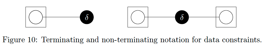
Data constraints are special because they denote observations. They also block any information flow across the edge in question [25]. Because they block information flow, CFFG notation optionally allows data constraints to terminate edges.

Here we wish to raise a subtle point about prior FFG notation. Previous work has used small black squares to denote data constraints following [21]. In keeping with our convention, a small black square on a CFFG denotes a $\delta$-distributed variable in the model $f$ rather than the variational distribution $q$. Being able to differentiate data constrained variables in $q$ and apriori fixed parameter of the model $f$ allows us to be explicit about what actually constitutes a data point for the inference problem at hand [caticha_entropic_2012].

In the case where ${\hat{v}}_j$ is not known,

• it can be treated as a parameter to be optimised.
• We refer to this case as a $\delta$-constraint or a pointmass constraint and
• notate it with an unfilled circle as shown in Fig 11

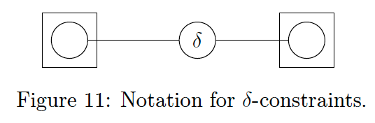
Unlike data constraints, the $\delta$-constraint allowsmessages to pass and is therefore not allowed to terminate an edge. Optimising the value of ${\hat{v}}_i$ under a $\delta$-constraint leads to EM as message passing [25].

5.4 Moment matching constraints

Moment matching constraints are special in that they replace the hard marginalisation constraints of Eq. (8) with constraints of the form

$$\begin{array}{}\text{(31)}& q(s_i)=\int q({\mathit{s}}_a)\text{d}{s}_{a\mathrm{\setminus }i}⟹\int q({\mathit{s}}_a){\mathbf{T}}_i(s_i)\text{d}{\mathit{s}}_a=\int q(s_i){\mathbf{T}}_i(s_i)\text{d}{s}_i\end{array}$$

where ${\mathbf{T}}_i(s_i)$ are the sufficient statistics of an exponential family distribution. This move loosens the marginalisation constraint by instead only requiring that the moments in question align. When taking the first variation and solving, one obtains the expectation propagation (EP) algorithm [18].

For notational purposes, moment matching constraints are unique in that they involve both an edge- and a node-marginal. That means the effects are not localised to a single bead. To indicate which beads are involved, we replace the solid lines between them with dashed lines instead.

We denote moment matching constraints by an E inside the corresponding edge-bead as shown in Fig 12. Choosing the edge-bead over the node-bead is an arbitrary decision made mainly for convenience.

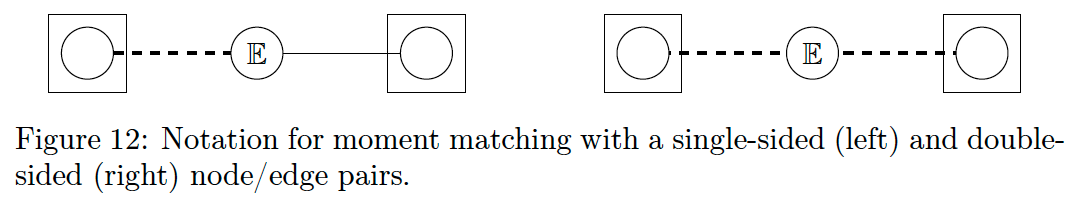
The left side of Fig. 12 shows notation for constraining a single node/edge pair by moment matching. If both nodes connected to an edge are under moment matching constraints, the double-sided notation on the right of Fig. 12 applies.

Given the modular nature of CFFG notation it is easy to compose different local constraints to accurately specify a Lagrangian and by extension an inference problem. Adding custom marginal constraints to a CFFG is also straightforward as it simply requires defining the meaning of a symbol inside a bead.

5.5 P-substitution on CFFGs

The final piece needed to represent the Active Inference Lagrangian on a CFFG is P-substitution. Being able to represent LAIF on a CFFG is the reason for constructing the local GFE using a mean-field factorisation and P-substitution. This construction is much more amenable to the tools we have developed so far as we will now demonstrate.

Recall that P-substitution involves substituting part of the model $p$ for $q$ in the expectation only. To write P-substitution on a CFFG, the logical notation is therefore to replace a circle with a square. Fig. 13 shows an example of adding a P-substitution to a mean-field factorised node marginal

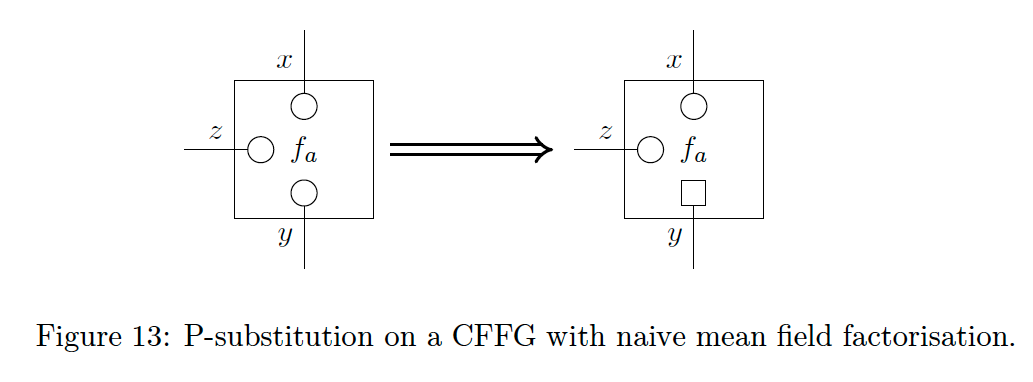
The square notation for P-substitution on CFFGs implies a conditioning of the P-substituted variable on all other connected variables that are not P-substituted. For example, in Fig. 13 the P-substitution changes local VFE to a GFE by

$$\begin{array}{}\text{(32)}& \begin{array}{r}\int \int \int \log \frac{q(y)q(x)q(z)}{p(y,x,z)}\stackrel{\text{from}}{\overbrace{q(y)}}q(x)q(z)\text{d}y\text{d}x\text{d}z\\ ⟹\int \int \int \log \frac{q(y)q(x)q(z)}{p(y,x,z)}\stackrel{\text{to}}{\overbrace{p(y\mid x,z)}}q(x)q(z)\text{d}y\text{d}x\text{d}z\end{array}\end{array}$$

Here, the P-substituted variable is $y$, and the remainder are $\{x,z\}$.

5.6 CFFG Compression

The value of CFFG notation is measured by how much it aids other researchers and practitioners in expressing their ideas accurately and succinctly. We envision two main groups for whom CFFGs might be of particular interest. The

• first group is comprised of mathematical researchers working on constrained free energy optimisation on FFGs. For this group we expect that the notation developed so far will be both useful and practically applicable since work is often focused on the intricacies of performing local optimisation. Commonly an FFG in this tradition is small but a very high level of accuracy is desired in order to be mathematically rigorous.

However there is a

• second group composed of applied researchers for whom the challenge is to accurately specify a

  • larger inference problem and its solution to solve an auxiliary goal - for instance controlling a drone, transmitting a coded message or simulating some phenomenon using AIF. For this group of researchers in particular,

  • CFFG notation as described so far might be too verbose and the overhead of using it may not outweigh the benefits gained. To this end,

  • we now complete CFFG notation by a mandatory compression step.

The compression step is designed to remove redundant information by enforcing an emphasis on deviations from a default BFE. By default, we mean no constraints other than normalisation and marginalisation and with a joint factorisation around every node. Recall that default normalisation constraints are denoted by empty, round beads and marginalisation by connected lines. A joint factorisation means all incoming edges are connected and the node only has a single, internal bead.

To provide a recipe for compressing a CFFG, we will need the concept of a bead chain. A

• bead chain is simply a
  • series of beads connected by edges. In the following recipe, a bead will only be summarised as part of a chain if it contains no additional information, meaning if it is round and empty.

To compress a CFFG, we follow a series of four steps:

1. Summarise every bead chain by their terminating beads.
2. For nodes with no factorisation constraints, remove empty, internal beads.
3. For nodes with no factorisation constraints, remove all internal edges.
4. For all factor nodes, push remaining internal beads to the border of the corresponding factor node.

After performing these steps, we are left with a compressed version of the original CFFG where each node can be much smaller and more concise. To exemplify, we apply the recipe to the CFFG in Fig. 14.

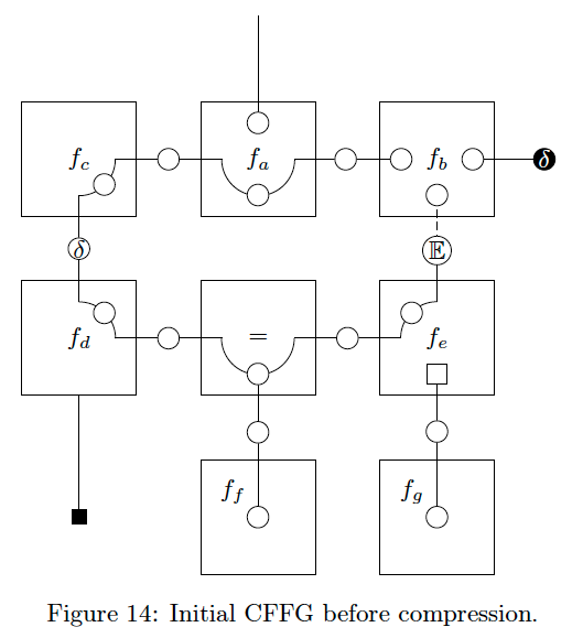
Fig. 14 is a complicated graph with loops, dangling edges, and multiple different factorisations in play. As a result, Fig. 14 covers a lot of special cases that one might encounter on a CFFG. We will now apply the steps in sequence, starting by removing empty beads on chains. This removes most of the beads in the inner loop as shown in Fig. 15

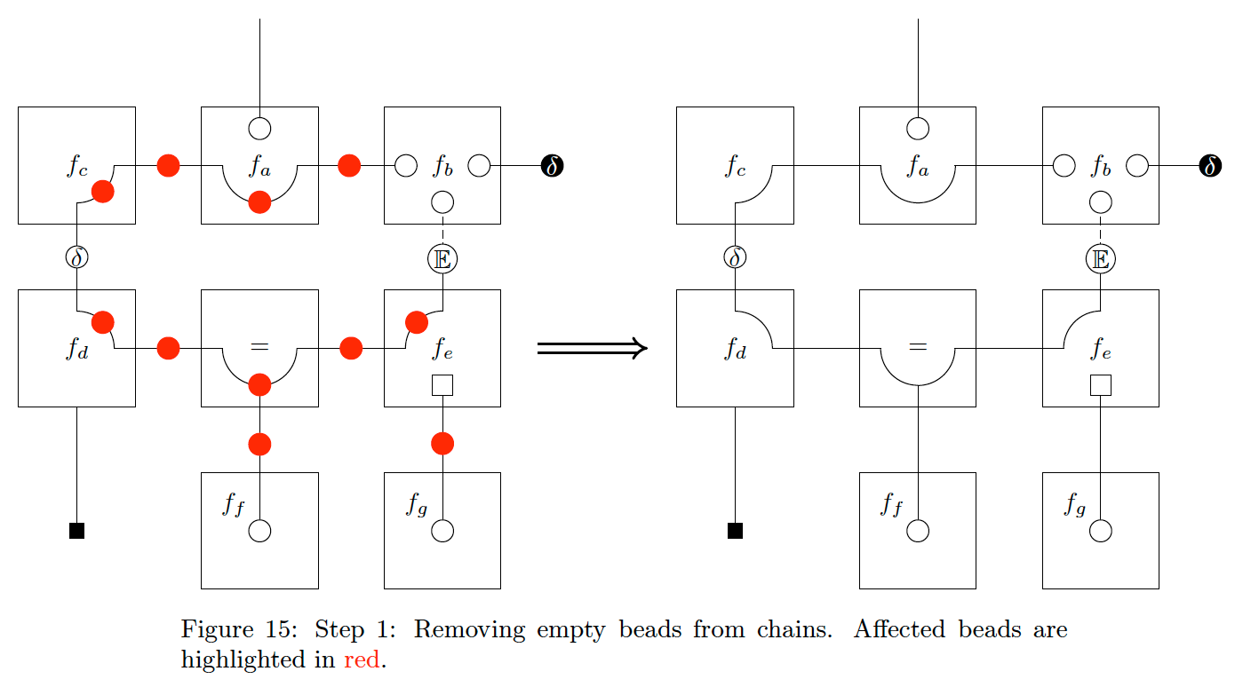
Note that the dangling edge extending from $f_a$ is treated as terminated by a bead and the bead on the edge is removed. Next, we remove any internal beads for nodes with no factorisation constraints. We show this step in Fig. 16

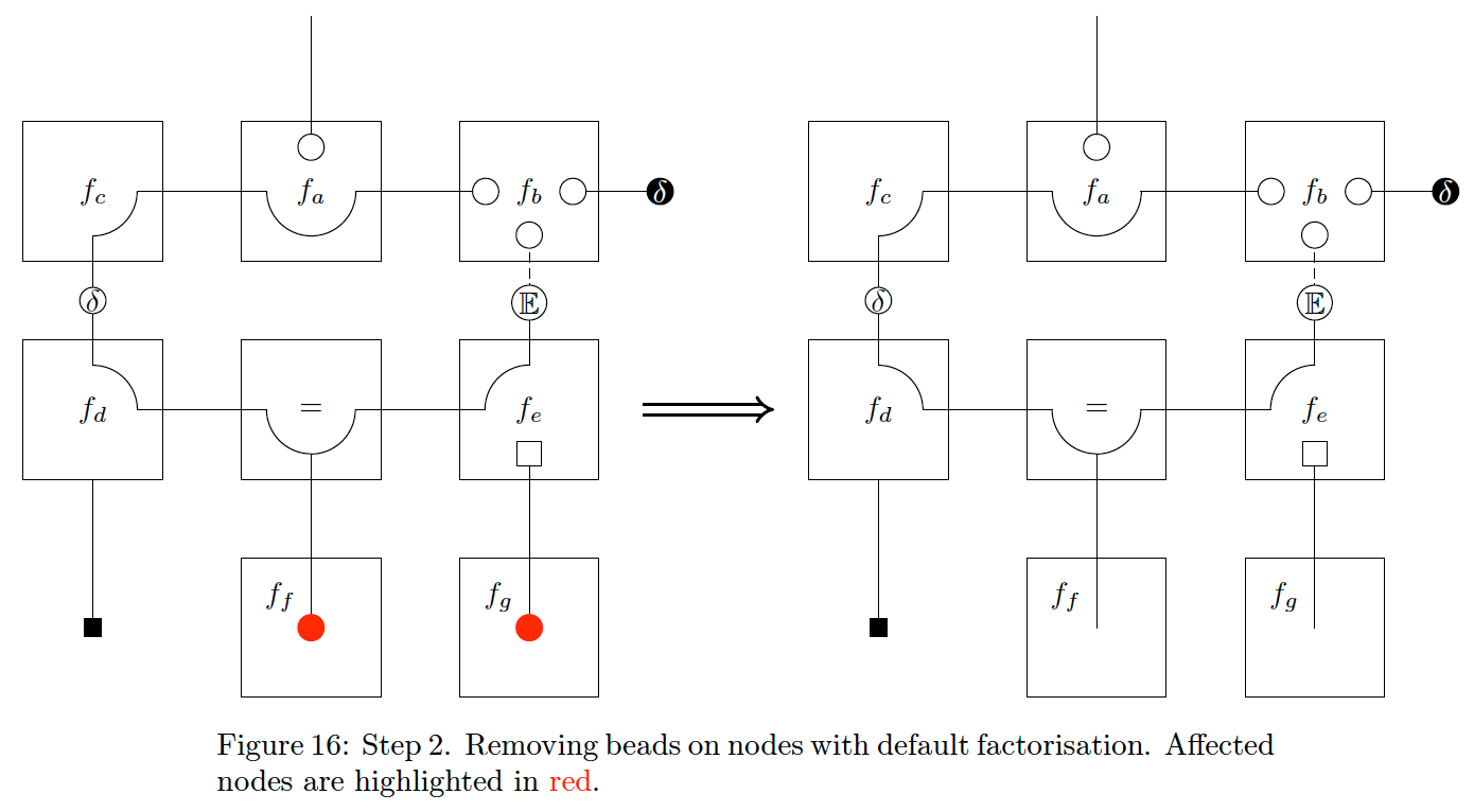
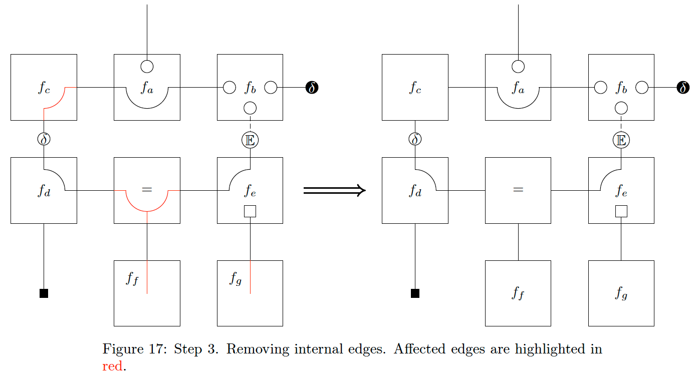
The next step is to remove any internal edge extensions for nodes with no factorisation constraints. We demonstrate this step in Fig. 17. Note that the internal edge of the node $f_d$ does not get cancelled since one of the connected edges is a pointmass in the model and therefore not present in $q$, meaning $f_d$ does not have a default factorisation.

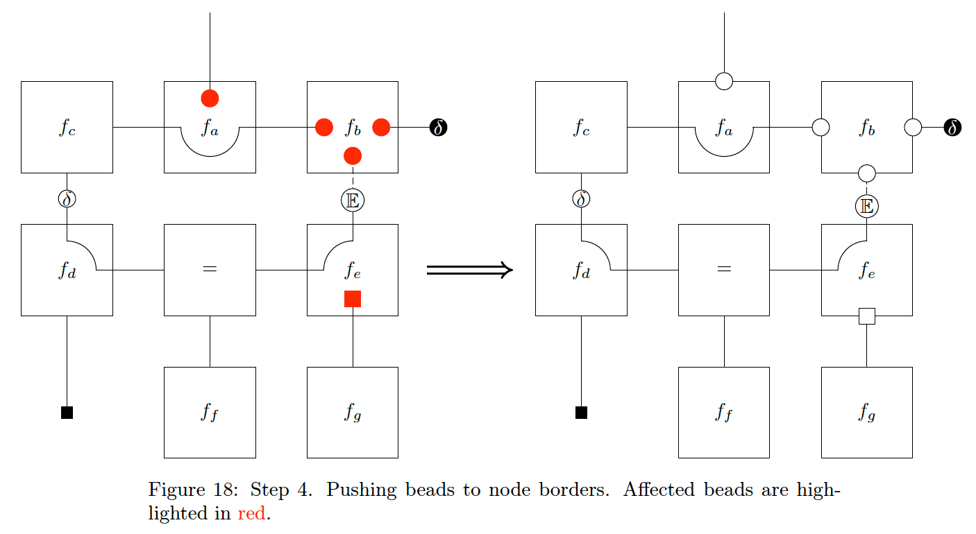
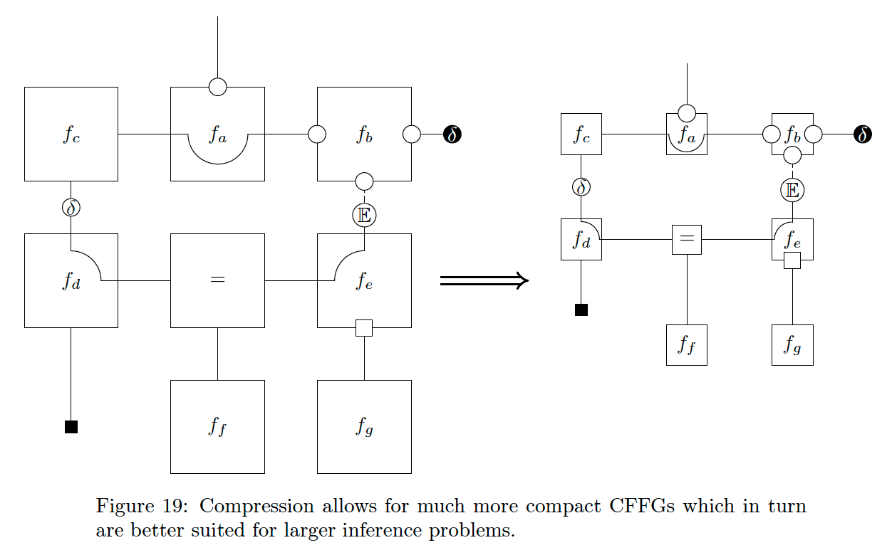
Finally, we can push any remaining internal beads to their node border, illustrated in Fig. 18. This step allows for writing the CFFG much more compactly, as we can see in Fig. 19.

At this point, we have removed most of the beads and edges and still retain most of the relevant information around all nodes. What is left is only what deviates from a default BFE specification {{i.e. all beads coincide-sedi}}. The goal here is, as stated initially, to make it easier to work with CFFG’s for larger models which necessitate working with smaller nodes.

From Fig. 19 it is clear that compression allows for much more compact CFFG’s which in turn are more amenable to larger CFFG’s. This is especially true in the

• absence of any factorisation or form constraints and P-substitutions in which case the
• compressed CFFG and underlying FFG are identical.

We see this with nodes $f_c$, $f_f$ , $f_g$ and $=$ in Fig. 19.

6 Classical AIF and the original GFE algorithm as special cases of LAIF

An integral part of working with MP algorithms is the choice of schedule - the order in which messages are passed. Many MP algorithms are iterative in nature and can therefore be sensitive to scheduling. LAIF is also an iterative MP algorithm and might consequently be sensitive to the choice of schedule.

A particularly interesting observation is that we can recover both the classical AIF planning algorithm of [6] and the scheme proposed by [19] as special cases of LAIF by carefully choosing the schedule and performing model comparison. This result extends upon prior work by [13] who reinterpreted the classical algorithm through the lens of MP on an FFG.

6.1 Example: CFFG and message updates for a discrete observation model with goals

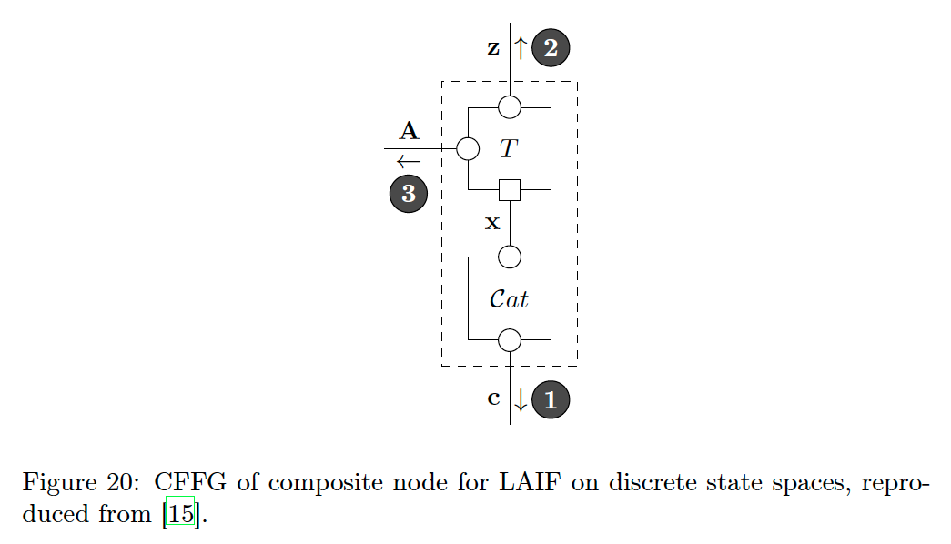
In order to both demonstrate LAIF and recover prior work, we need to derive the required messages. We refer to our companion paper [15] for the detailed derivations and summarise the results here. For the remaining paragraphs, we will use $\mathbf{x}$ to denote that $x$ is vector-valued and $\mathbf{A}$ to denote that $A$ is either a matrix or a tensor. For the discrete case, we work with a composite node corresponding to the factor

$$\begin{array}{rl}p(\mathbf{x}\mid \mathbf{A}\mathbf{,}\mathbf{s})& =\mathcal{Cat}(\mathbf{x}\mid \mathbf{A}\mathbf{s})(33a)\\ p^{+}(\mathbf{x}\mid \mathbf{c})& =\mathcal{Cat}(\mathbf{x}\mid \mathbf{c})(33b)\end{array}$$

We show the corresponding CFFG in Fig. 20 where we indicate the necessary factorisation and P-substitution. In the parlance of AIF Eq. 33a defines a model composed of a discrete state transition $(T)$ with transition matrix $\mathbf{A}$ and a categorical goal prior ($\mathcal{Cat}$) with parameter vector $\mathbf{c}$. Before stating the messages, we define the vector

$$\begin{array}{}\text{(34)}& \mathbf{h}(\mathbf{A})=-\text{diag}({\mathbf{A}}^T\text{log}\mathbf{A})\end{array}$$

This term is often denoted $\mathbf{H}$ in other works [4, 19]. We instead opt for using lowercase since the term is a vector and for making the dependence on $\mathbf{A}$ explicit. In the following section, we will sometimes use an overbar to denote expectations, such that ${\mathbb{E}}_{q(x)}[g(x)]=\overline{g(x)}$. Additionally, we define

$$\begin{array}{rl}\xi (\mathbf{A})& =({\mathbf{A}}^{\text{T}})(\overline{\text{log}\mathbf{c}}-\text{log}(\bar{\mathbf{A}}\bar{\mathbf{z}})-\mathbf{h}(\mathbf{A})(35a)\\ \rho & =({\bar{\mathbf{A}}}^{\text{T}})(\overline{\text{log}\mathbf{c}}-\text{log}(\bar{\mathbf{A}}\bar{\mathbf{z}})-\overline{\mathbf{h}(\mathbf{A})}(35b)\end{array}$$

in order to make the expressions more concise. Where expectations cannot be computed in closed form, we instead resort to Monte Carlo estimates. With this notation in place, we can write the required messages as

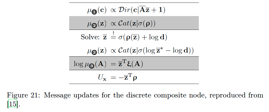
Fig. 21 shows the message updates towards all connected variables as well as the average energy term ($U_x$) for the composite node. $\mathbf{d}$ denotes the parameters of the incoming message from the rest of the CFFG on the edge $z$. Interestingly, the energy term $U_x$ corresponds exactly to the EFE as used in standard AIF [4, 6].

Special attention needs to be given to the messages ${\mu }_2(\mathbf{z})$ and ${\mu }_3(\mathbf{A})$. While ${\mu }_2(\mathbf{z})$ can be solved for in closed form, in practice applying this result directly can lead to unstable solutions that fluctuate between multiple extrema. For this reason, we opt for parameterising the message by $\bar{\mathbf{z}}$ and solving for parameters of the marginal directly using Newton’s method. Having found the optimum ${\bar{\mathbf{z}}}^{\ast }$ we can then substitute the result into the message expression to obtain a stable solution.

The message ${\mu }_3(\mathbf{A})$ does not follow a nice exponential family distribution. To circumvent this problem, we can pass on the logpdf directly. When we need to compute the marginal $q(\mathbf{A})$, we can then use sampling procedures to estimate the necessary expectations [1]. Further details and full derivations can be found in our companion paper [15].

6.2 Reconstructing classical AIF

With our new messages in hand and equipped with CFFG notation, we can now restate prior work unambiguously, starting with the classical algorithm of [6]. To reconstruct the algorithm of [6], we start by defining the generative model. The generative model is a discrete partially observed Markov decision process (POMDP) over future time steps given by

$$\begin{array}{}\text{(36)}& \begin{array}{rl}p(\underset{\text{Future}}{\underbrace{{\mathbf{x}}_{t+1:T},{\mathbf{s}}_{t:T}}}\mid \underset{\text{Policy}}{\underbrace{{\hat{\mathbf{u}}}_{t+1:T}}},\underset{\text{Past}}{\underbrace{{\mathbf{x}}_{1:t},{\mathbf{u}}_{1:t}}})& \propto \underset{\text{State Prior}}{\underbrace{p({\mathbf{s}}_t\mid {\mathbf{x}}_{1:t},{\mathbf{u}}_{1:t})}}\prod _{k=t+1}^T\underset{\text{Likelihood}}{\underbrace{p({\mathbf{x}}_k\mid {\mathbf{s}}_k)}}\underset{\text{State Transition}}{\underbrace{p({\mathbf{s}}_k\mid {\mathbf{s}}_{k-1},{\hat{\mathbf{u}}}_k}}\underset{\text{Goal Prior}}{\underbrace{p^{+}({\mathbf{x}}_k)}}\end{array}\end{array}$$

where

$$\begin{array}{rl}p({\mathbf{s}}_t\mid {\mathbf{x}}_{1:t},{\mathbf{u}}_{1:t})& =\mathcal{Cat}({\mathbf{s}}_t\mid \mathbf{d})(37)\\ p({\mathbf{s}}_k\mid {\mathbf{s}}_{k-1},{\hat{\mathbf{u}}}_k& =\mathcal{Cat}({\mathbf{s}}_k\mid {\mathbf{B}}_{{\hat{u}}_k}{\mathbf{s}}_{k-1})(38)\\ p({\mathbf{x}}_k\mid {\mathbf{s}}_k)& =\mathcal{Cat}({\mathbf{x}}_k\mid \mathbf{A}{\mathbf{s}}_k)(39)\\ p^{+}({\mathbf{x}}_k)& =\mathcal{Cat}({\mathbf{x}}_k\mid {\mathbf{c}}_k)(40)\end{array}$$

Here we let ${\mathbf{x}}_k$ denote observations, ${\mathbf{z}}_k$ latent states, and ${\hat{\mathbf{u}}}_k$ a fixed control, with the subscript $k$ indicating the future time step in question. The initial state zt represents the filtering solution given the agents trajectory so far which we summarise in the parameter vector $\mathbf{d}$. Control signals correspond to particular transition matrices ${\mathbf{B}}_{{\hat{u}}_k}$ where we use the subscript to emphasize that each $\mathbf{B}$ matches a particular control ${\hat{\mathbf{u}}}_k$. The observation model is given by the known matrix $\mathbf{A}$. Note that Eq. (36) is not normalised as it includes goal priors over $\mathbf{x}$. The CFFG of (36) is shown in Fig 22.

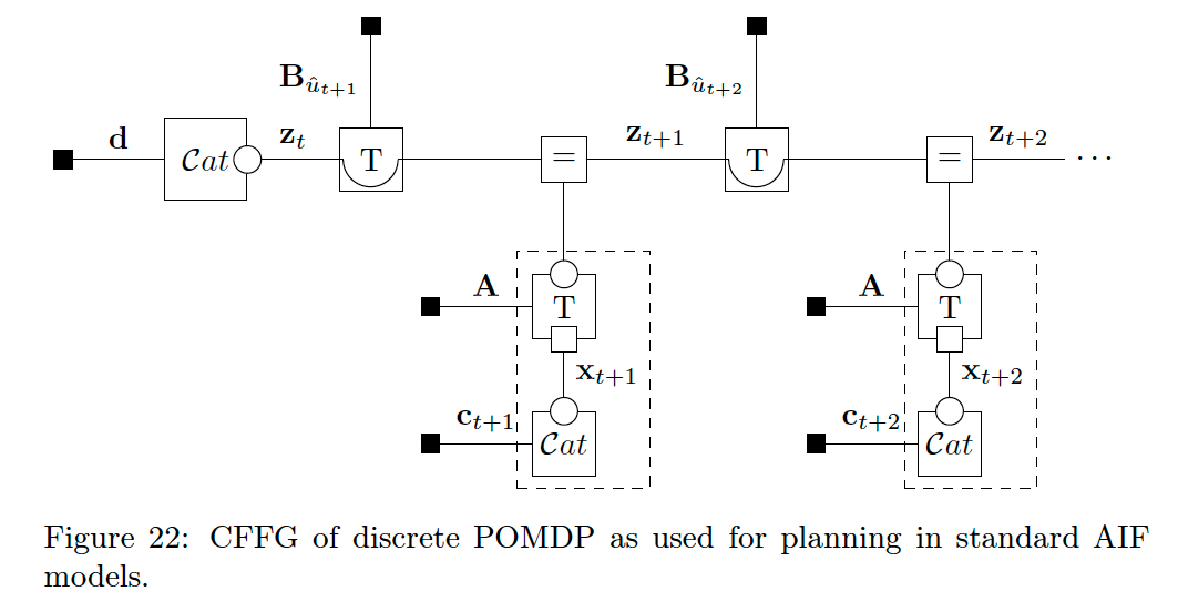
where $\text{T}$ nodes denote a discrete state transition (multiplication of a categorical variable by a transition matrix {{probability matrix ?}}). Given a generative model with a fixed set of controls, the next step is to compute the EFE [4, 6, 13, 14]. We provide a brief description here and refer to Appendix A and [4, 13, 14, 22] for more detailed descriptions. The EFE is given by

$$\begin{array}{}\text{(41)}& G({\hat{\mathbf{u}}}_{t+1:T})=\sum _{k=t}^T\int \int \text{log}\frac{q({\mathbf{s}}_k\mid {\hat{\mathbf{u}}}_k)}{p({\mathbf{x}}_k,{\mathbf{s}}_k\mid {\hat{\mathbf{u}}}_k)}p({\mathbf{x}}_k\mid {\mathbf{s}}_k)q({\mathbf{s}}_k\mid {\hat{\mathbf{u}}}_k)\text{d}{\mathbf{x}}_k\text{d}{\mathbf{s}}_k\end{array}$$

With a slight abuse of notation, we can compute EFE by first applying transition matrices to the latent state and generating predicted observations as

$$\begin{array}{}\text{(42)}& \begin{array}{rl}{\mathbf{s}}_k& ={\mathbf{B}}_{{\hat{u}}_k}{\mathbf{s}}_{k-1}\\ {\mathbf{x}}_k& =\mathbf{A}{\mathbf{s}}_k\end{array}\end{array}$$

{{Why not simply have:}}

$$\begin{array}{rl}{\mathbf{s}}_k& \sim {\mathbf{B}}_{{\hat{u}}_k}{\mathbf{s}}_{k-1}\\ {\mathbf{x}}_k& \sim \mathbf{A}{\mathbf{s}}_k\end{array}$$

In Eq. (42) we slightly abuse notation by having ${\mathbf{s}}_k$ (resp. ${\mathbf{x}}_k$) refer to the prediction after applying the transition matrix ${\mathbf{B}}_{{\hat{u}}_k}$ (resp. $\mathbf{A}$) instead of the random variable as we have done elsewhere.

We can recognise these operations as performing a forwards MP sweep using belief propagation messages. With this choice of generative model, the EFE of a policy ${\hat{\mathbf{u}}}_{t+1:T}$ is found by [4, Eq. D.2-3]

$$\begin{array}{}\text{(43)}& G({\hat{\mathbf{u}}}_{t+1:T})=\sum _{k=t+1}^T-\text{diag}({\mathbf{A}}^T\text{log}\mathbf{A}{)}^T{\mathbf{s}}_k+{\mathbf{x}}_k^T(\text{log}{\mathbf{x}}_k-\text{log}{\mathbf{c}}_k)\end{array}$$

where ${\mathbf{c}}_k$ denotes the parameter vector {{i.e. probability vector}} of a goal prior at the $k$’th time step. To select a policy we simply pick the sequence ${\hat{\mathbf{u}}}_{t+1:T}$ that results in the lowest numerical value when solving Eq. (43).

To write this method on the CFFG in Fig. 22, we can simply add messages to the CFFG and note that the sum of energy terms of the P-substituted composite nodes in Fig. 21 matches Eq. (43). We show this result in Fig. 23.

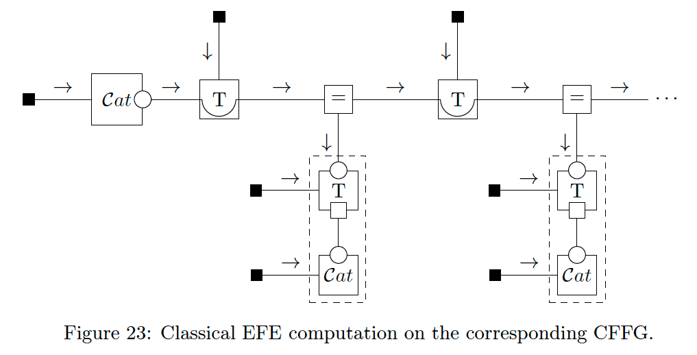
Comparing different policies (choices of ${\hat{\mathbf{u}}}_{t+1:T}$) and computing the energy terms of the P-substituted composite nodes is then exactly equal to the EFE-computation detailed in [6].

6.3 Reconstructing the original GFE method

We can further exemplify the capabilities of CFFG notation by recapitulating the update rules given in the original GFE paper [19]. To recover the procedure of [19], we need to extend the generative model to encompass past observations as

$p({\mathbf{x}}_{1:T},{\mathbf{s}}_{0:T}\mid {\hat{\mathbf{u}}}_{1:T})$ $$\begin{array}{}\text{(44)}& \begin{array}{r}\propto p({\mathbf{s}}_0)\underset{\text{Past}}{\underbrace{\prod _{l=1}^{t}p({\mathbf{x}}_l\mid {\mathbf{s}}_l)p({\mathbf{s}}_l\mid {\mathbf{s}}_{l-1},{\hat{\mathbf{u}}}_l)}}\underset{\text{Future}}{\underbrace{\prod _{k=t+1}^{T}p({\mathbf{x}}_k\mid {\mathbf{s}}_k)p({\mathbf{s}}_k\mid {\mathbf{s}}_{k-1},{\hat{\mathbf{u}}}_k)\stackrel{\text{Goal prior}}{\overbrace{p^{+}({\mathbf{x}}_k)}}}}\end{array}\end{array}$$

where

$$\begin{array}{}\text{(45)}& \begin{array}{rl}p({\mathbf{s}}_0)& =\mathcal{Cat}({\mathbf{s}}_0\mid \mathbf{d})\\ p({\mathbf{s}}_t\mid {\mathbf{s}}_{t-1},{\hat{\mathbf{u}}}_t& =\mathcal{Cat}({\mathbf{s}}_t\mid {\mathbf{B}}_{{\hat{u}}_t}{\mathbf{s}}_{t-1})\\ p({\mathbf{x}}_t\mid {\mathbf{s}}_t)& =\mathcal{Cat}({\mathbf{x}}_t\mid \mathbf{A}{\mathbf{s}}_t)\\ p^{+}({\mathbf{x}}_k)& =\mathcal{Cat}({\mathbf{x}}_k\mid {\mathbf{c}}_k)\end{array}\end{array}$$

For past time steps, we add data constraints and for future time steps we perform P-substitution. We also apply a naive mean field factorisation for every node. The final ingredient we need is a schedule that includes both forwards and backwards passes as hinted at in [13]. For $t=1$ the corresponding CFFG is shown in Fig. 24 with messages out of the P-substituted nodes highlighted in red. These messages are given by ${\mu }_2(\mathbf{s})$ in Fig. 24.

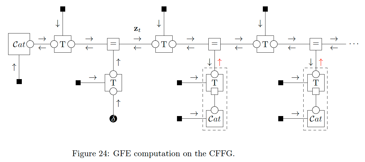
With these choices, the update equations become identical to those of [19]. Indeed, careful inspection of the update rules given in [19] reveals the component parts of the P-substituted message. However, by using CFFGs and P-substitution, we can cast their results as MP on generic graphs which immediately generalises their results to free-form graphical models.

Once inference has converged, we note that [19] shows that GFE evaluates identically to the EFE, meaning we can use the same model comparison procedure to select between policies as we used for reconstructing the classical algorithm. This shows how we can obtain the algorithm of [19] as a special case of LAIF.

7 LAIF for policy inference

The tools presented in this chapter are not limited to restating prior work. Indeed, LAIF offers several advantages over prior methods, one of which is the ability to directly infer a policy instead of relying on a post hoc comparison of energy terms.

• To demonstrate, we solve two variations of the classic T-maze task [6].

This is a well-studied setting within the AIF literature and therefore constitutes a good minimal benchmark. In the

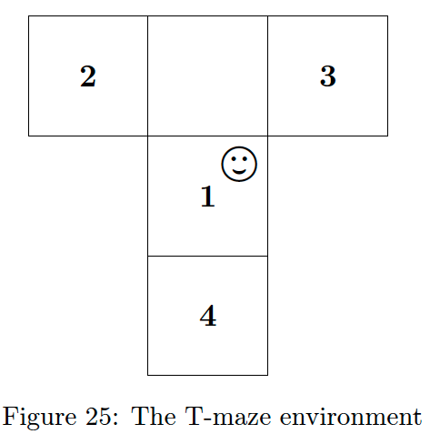
• T-maze experiment, the agent lives in a maze with four locations as depicted in Fig. 25. The

  • agent starts in position 1 and knows that a
  • reward is present at either position 2 or 3, but not which one. At
  • position 4 is a cue that informs the agent which arm contains the reward.

The optimal action to take is therefore to first visit 4 and learn which arm contains the reward before going to the rewarded arm. Because this course of action requires delaying the reward, an agent following a greedy policy behaves sub-optimally. The T-maze is therefore considered a reasonable minimal example of the epistemic, information-seeking behaviour that is a hallmark of AIF agents. We implemented our experiments in the reactive MP toolbox RxInfer [2]. The source code for our simulations is available at https://github.com/biaslab/LAIF.

7.1 Model specification

The generative model for the $\text{T}$-maze is an adaptation of the discrete POMDP used by [6, 19]. We assume the agent starts at some current timestep t and want to infer a policy up to a known time horizon $T$. The generative model is then

$$\begin{array}{}\text{(46)}& \begin{array}{rl}p(\mathit{x},\mathit{s},\mathit{u})& \propto \underset{\begin{array}{c}\text{Initial}\\ \text{state}\\ \text{prior}\end{array}}{\underbrace{p({\mathbf{s}}_0)}}\prod _{k=t+1}^T\underset{\begin{array}{c}\text{Observation}\\ \text{model}\end{array}}{\underbrace{p({\mathbf{x}}_k\mid {\mathbf{s}}_k)}}\underset{\begin{array}{c}\text{Transition}\\ \text{model}\end{array}}{\underbrace{p({\mathbf{s}}_k\mid {\mathbf{s}}_{k-1},{\mathbf{u}}_k}})\underset{\begin{array}{c}\text{Control}\\ \text{prior}\end{array}}{\underbrace{p({\mathbf{u}}_k)}}\underset{\begin{array}{c}\text{Goal}\\ \text{prior}\end{array}}{\underbrace{p^{+}({\mathbf{x}}_k)}}\end{array}\end{array}$$

where

$$\begin{array}{rl}p({\mathbf{s}}_t)& =\mathcal{Cat}({\mathbf{s}}_0\mid \mathbf{d})(47a)\\ p({\mathbf{x}}_k\mid {\mathbf{s}}_k)& =\mathcal{Cat}({\mathbf{x}}_k\mid \mathbf{A}{\mathbf{s}}_k)(47b)\\ p({\mathbf{s}}_k\mid {\mathbf{s}}_{k-1},{\mathbf{u}}_k)& =\prod _{\kappa }[\mathcal{Cat}({\mathbf{s}}_k\mid {\mathbf{B}}_{\kappa }{\mathbf{s}}_{k-1}){]}^{{\mathbf{u}}_{\kappa k}}(47c)\\ & =\mathcal{Cat}({\mathbf{s}}_k\mid {\mathbf{B}}_{u_k}{\mathbf{s}}_{k-1})\\ p({\mathbf{u}}_k)& =\mathcal{Cat}({\mathbf{u}}_k\mid {\mathbf{e}}_k)(47d)\\ p^{+}({\mathbf{x}}_k)& =\mathcal{Cat}({\mathbf{x}}_k\mid {\mathbf{c}}_k)(47e)\end{array}$$

{{In general:}}

• $n,t$ for time
• $k$ for future time
• $l$ for past time
• $\kappa$ for ’k’omponent, ’k’lass or ’k’andidate of a mixture

${\mathbf{u}}_k$ is a one-hot encoded vector of length $\kappa$. The notation ${\mathbf{u}}_{\kappa k}$ picks the $\kappa$’th entry of ${\mathbf{u}}_k$. We show the corresponding CFFG in Fig 26.

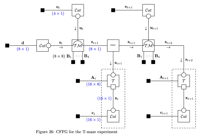
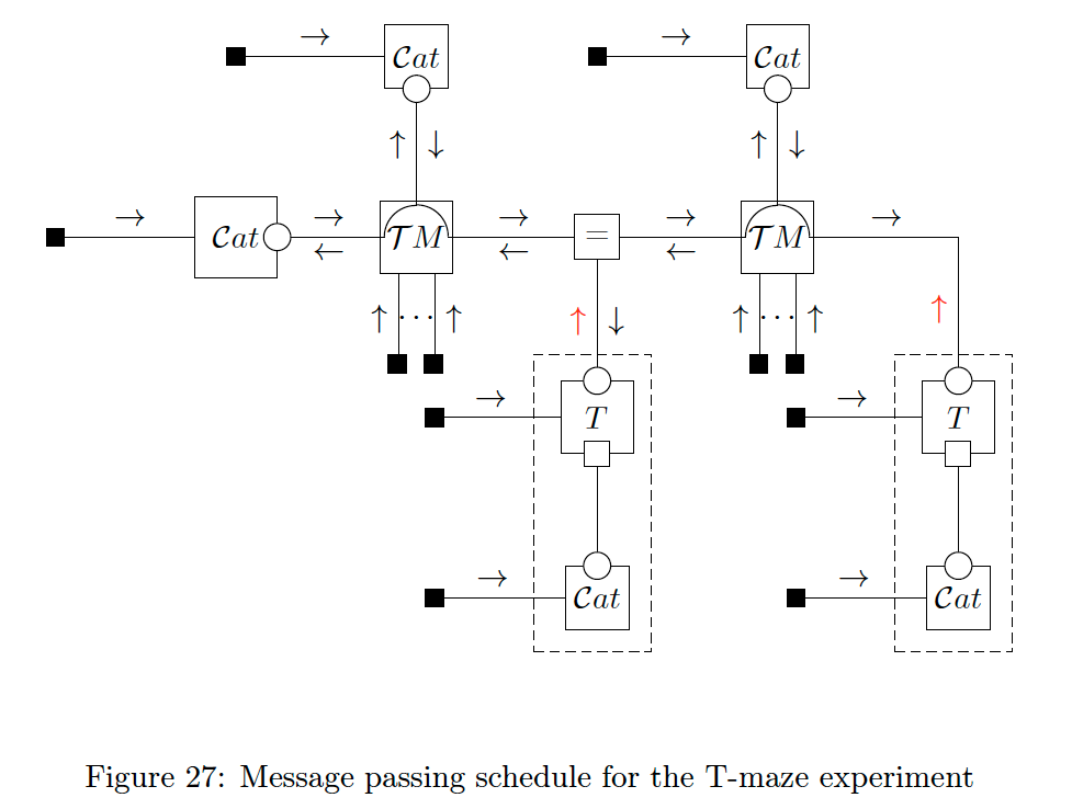
Eq. (47c) defines a mixture model over candidate transition matrices indexed by ${\mathbf{u}}_k$. We give the details of this node function and the required messages in Appendix C. The MP schedule is shown in Fig. 27 with GFE-based messages highlighted in red

Following [6] we define the initial state and control prior as

$$\begin{array}{}\text{(48a)}& \mathbf{d}=\underset{\text{RL, RR}}{\underbrace{(0.5,0.5{)}^T}}\otimes \underset{\text{O, L, R, C}}{\underbrace{(1,0,0,0{)}^T}}\end{array}$$ $$\begin{array}{}\text{(48b)}& {\mathbf{e}}_k=(0.25,0.25,0.25,0.25)\mathrm{\forall }k\end{array}$$

with $\otimes$ denoting the Kronecker product. {{The factors were swapped to align with the code implementation (confirmed with Magnus Koudahl)}} The transition mixture node requires a set of candidate transition matrices. The T-maze utilises four possible transitions, given below

$${\mathbf{B}}_1=\left[\begin{array}{cccc}1& 1& 1& 1\\ 0& 0& 0& 0\\ 0& 0& 0& 0\\ 0& 0& 0& 0\end{array}\right]\otimes {\mathbf{I}}_2,{\mathbf{B}}_2=\left[\begin{array}{cccc}0& 1& 1& 0\\ 1& 0& 0& 1\\ 0& 0& 0& 0\\ 0& 0& 0& 0\end{array}\right]\otimes {\mathbf{I}}_2$$

$$\begin{array}{}\text{(49)}& {\mathbf{B}}_3=\left[\begin{array}{cccc}0& 1& 1& 0\\ 0& 0& 0& 0\\ 1& 0& 0& 1\\ 0& 0& 0& 0\end{array}\right]\otimes {\mathbf{I}}_2,{\mathbf{B}}_4=\left[\begin{array}{cccc}0& 1& 1& 0\\ 0& 0& 0& 0\\ 0& 0& 0& 0\\ 1& 0& 0& 1\end{array}\right]\otimes {\mathbf{I}}_2\end{array}$$

where ${\mathbf{I}}_2$ denotes a 2×2 identity matrix. Note that these differ slightly from the original implementation of [6]. In [6] invalid transitions are represented by an identity mapping where we instead model invalid transitions by sending the agent back to position 1. The likelihood matrix $\mathbf{A}$ is given by four blocks, corresponding to the observation likelihood in each position.

$$\begin{array}{}\text{(50)}& \mathbf{A}=\left[\begin{array}{cccc}{\mathbf{A}}_1& & & \\ & {\mathbf{A}}_2& & \\ & & {\mathbf{A}}_3& \\ & & & {\mathbf{A}}_4\end{array}\right]\end{array}$$

with everything outside the blocks being set to 0. The blocks are

$${\mathbf{A}}_1=\left[\begin{array}{cc}0.5& 0.5\\ 0.5& 0.5\\ 0& 0\\ 0& 0\end{array}\right],{\mathbf{A}}_2=\left[\begin{array}{cc}0& 0\\ 0& 0\\ \alpha & 1-\alpha \\ 1-\alpha & \alpha \end{array}\right]$$

$$\begin{array}{}\text{(51)}& {\mathbf{A}}_3=\left[\begin{array}{cc}0& 0\\ 0& 0\\ 1-\alpha & \alpha \\ \alpha & 1-\alpha \end{array}\right],{\mathbf{A}}_4=\left[\begin{array}{cc}1& 0\\ 0& 1\\ 0& 0\\ 0& 0\end{array}\right]\end{array}$$

with $\alpha$ being the probability of observing a reward. The goal prior is given by

$$\begin{array}{}\text{(52)}& {\mathbf{c}}_k=\underset{\text{CL, CR, RW, NR}}{\underbrace{\sigma ((0,0,c,-c{)}^T}}\otimes \underset{\text{O, L, R, C}}{\underbrace{(1,1,1,1{)}^T)}}\mathrm{\forall }k\end{array}$$

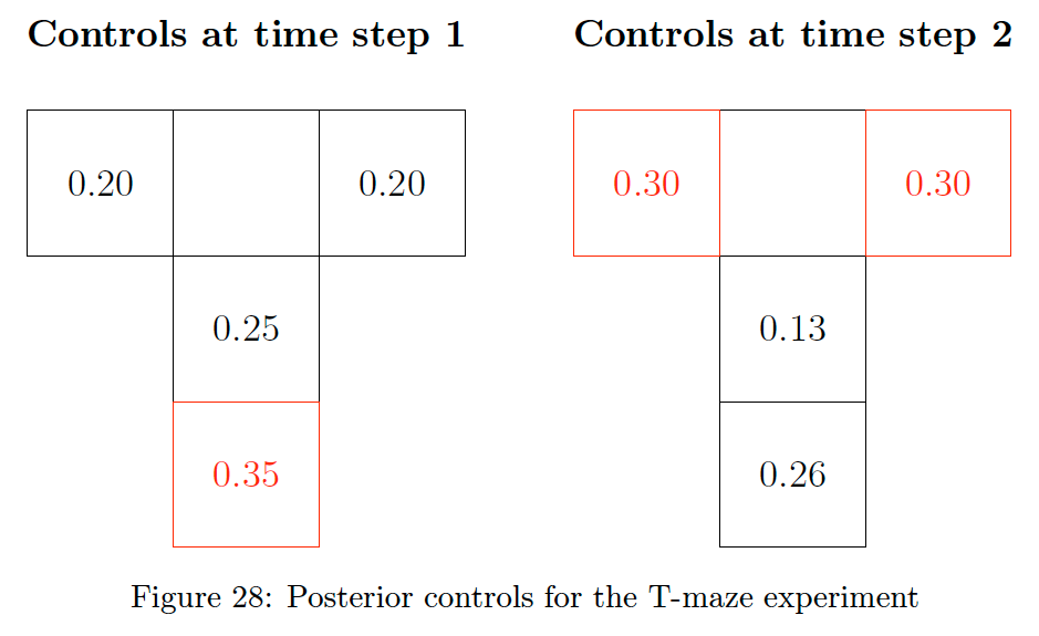
with $c$ being the utility ascribed to a reward and $\sigma (·)$ the softmax function. Inference for the parts of the model not in $\mathcal{P}$ can be accomplished using belief propagation. We follow the experimental setup of [6] and let $c=2,\alpha =0.9$. For inference, we perform two iterations of our MP procedure and use 20 Newton steps to obtain the parameters of the outgoing message from the P-substituted nodes.

We show the results in Fig. 28. The number in each cell is the posterior probability mass assigned to the corresponding action, with the most likely actions highlighted in red.

Fig. 28 shows an agent that initially prefers the epistemic action (move to state 4) at time $t+1$ and subsequently exhibits a preference for either of then potentially rewarding arms (indifferent between states 2 and 3). This shows that LAIF is able to infer the optimal policy and that our approach can reproduce prior results on the T-maze.

Since CFFGs are inherently modular, they allow us to modify the inference task without changing the model. To demonstrate, we now add  -constraints to the control variables. This corresponds to selecting the MAP estimate of the control posterior [25] and results in the CFFG shown in Fig. 29. The schedule and all messages remain the same as our previous experiment - however now the agent will select the most likely course of action instead of providing us with a posterior distribution.

Performing this experiment yields the policy shown in Fig. 30

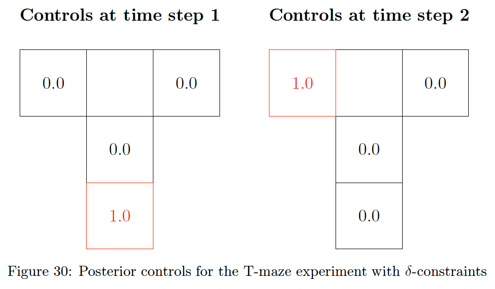
Fig. 30 once again shows that the agent is able to infer the optimal policy for solving the task. For repeated runs, the agent will randomly select to move to either position 2 or 3 at the second step due to minute differences in the Monte Carlo estimates used for computing the messages. The pointmass constraint obscures this since it forces the marginal to put all mass on the MAP estimate.

The point of repeating the experiments with  -constraints is not to show that the behaviour of the agent changes dramatically. Instead, the idea is to demonstrate that CFFGs allow for modular specification of AIF agents which allows for adapting parts of the model without having to touch the rest. In this case, the only parts of inference that change are those involving the control marginal. This means all messages out of the P-substituted composite nodes are unaffected since the $\delta$-constraints are only applied to the control marginals.

8 Conclusions

In this paper we have proposed a novel approach to AIF based on lagrangian optimisation which we have named Lagrangian Active Inference (LAIF). We demonstrated LAIF on a classic benchmark problem from the AIF literature and found that it inherits the epistemic drive that is a hallmark feature of AIF. LAIF presents three main advantages over previous algorithms for AIF.

• Firstly, an advantage of LAIF is the computational efficiency afforded by being able to pass backward messages instead of needing to perform forwards rollouts for every policy. While LAIF is still an iterative procedure, the computational complexity of each iteration scales linearly in the size of the planning horizon T instead of exponentially.
• A second advantage is that LAIF allows for directly inferring posteriors over control signals instead of relying on a model comparison step based on EFE/GFE. This means that LAIF unifies inference for perception, learning, and actions into a single procedure without any overhead - it all becomes part of the same inference procedure. See our companion paper [15] for more details.
• Thirdly, LAIF is inherently modular and consequently works for freely definable CFFGs, while prior work has focused mostly on specific generative models. Extensions to hierarchical or heterarchical models are straightforward and only require writing out the corresponding CFFG.

We have also introduced CFFG notation for writing down constraints and P-subtitutions on an FFG. CFFGs are useful not just for AIF but for specifying free energy functionals in general. CFFGs accomplish this through a simple and intuitive graphical syntax. Our hope is that CFFGs can become a standard tool similar to FFGs when it is desirable to write not just a model $f$ but also a family of approximating distributions $\mathcal{Q}$. Specifically in the context of AIF we have also introduced P-substitution as a way to modify the underlying free energy functional. In doing so we have formalised the relation between AIF and message passing on a CFFG, paving the way for future developments.

In future work, we plan to extend LAIF to more node constructions to further open up the scope of available problems that can be attacked using AIF.

References

[1] Semih Akbayrak, Ivan Bocharov, and Bert de Vries. “Extended variational message passing for automated approximate Bayesian inference”. In: En- tropy 23.7 (2021), p. 815.

[2] Dmitry Bagaev and Bert de Vries. “Reactive Message Passing for Scalable Bayesian Inference”. en. In: (2022). Submitted to the Journal of Machine Learning Research.

[3] Théophile Champion et al. “Branching Time Active Inference: The theory and its generality”. In: Neural Networks 151 (2022), pp. 295–316. issn: 0893-6080. doi: https://doi.org/10.1016/j.neunet.2022.03.036. url: https://www.sciencedirect.com/science/article/pii/S0893608022001149.

[4] Lancelot Da Costa et al. “Active inference on discrete state-spaces: a synthesis”. en. In: arXiv:2001.07203 [q-bio] (Jan. 2020). arXiv: 2001.07203. url: http://arxiv.org/abs/2001.07203 (visited on 01/22/2020).

[5] Karl Friston. “A free energy principle for a particular physics”. In: arXiv:1906.10184 [q-bio] (June 2019). arXiv: 1906.10184. url: http://arxiv.org/abs/1906.10184 (visited on 06/12/2020).

[6] Karl Friston et al. “Active inference and epistemic value”. In: Cogni- tive Neuroscience 6.4 (Oct. 2015), pp. 187–214. issn: 1758-8928. doi: 10.1080/17588928.2015.1020053. url: https://doi.org/10.1080/17588928.2015.1020053 (visited on 09/09/2019).

[7] Karl Friston et al. “Sophisticated Inference”. In: Neural Computation 33.3 (Mar. 2021), pp. 713–763. issn: 0899-7667. doi: 10.1162/neco_a_01351. url: https://doi.org/10.1162/neco_a_01351 (visited on 12/22/2021).

[8] Karl J. Friston et al. “Action and behavior: a free-energy formulation”. en. In: Biological Cybernetics 102.3 (Mar. 2010), pp. 227–260. issn: 0340-1200, 1432-0770. doi: 10.1007/s00422-010-0364-z. url: http://link.springer.com/10.1007/s00422-010-(visited on 04/13/2020).

[9] Karl J. Friston et al. SPM12 toolbox, http://www.fil.ion.ucl.ac.uk/spm/software/. 2014.

[10] Danijar Hafner et al. “Action and Perception as DivergenceMinimization”. In: arXiv:2009.01791 [cs, math, stat] (Oct. 2020). arXiv: 2009.01791. url: http://arxiv.org/abs/2009.01791 (visited on 01/07/2021).

[11] Conor Heins et al. “pymdp: A Python library for active inference in discrete state spaces”. In: arXiv preprint arXiv:2201.03904 (2022).

[12] Hilbert J. Kappen, Vicenç Gómez, and Manfred Opper. “Optimal control as a graphical model inference problem”. en. In: Machine Learning 87.2 (May 2012), pp. 159–182. issn: 0885-6125, 1573-0565. doi: 10.1007/s10994-012-5278-7. url: http://link.springer.com/10.1007/s10994-012-5278-7 (visited on 02/07/2020).

[13] Magnus Koudahl, Christopher L Buckley, and Bert de Vries. “A Message Passing Perspective on Planning Under Active Inference”. In: Active Inference: Third International Workshop, IWAI 2022, Grenoble, France, September 19, 2022, Revised Selected Papers. Springer. 2023, pp. 319–327.

[14] Magnus T. Koudahl,Wouter M. Kouw, and Bert de Vries. “On Epistemics in Expected Free Energy for Linear Gaussian State Space Models”. In: En- tropy 23.12 (Nov. 2021), p. 1565. issn: 1099-4300. doi: 10.3390/e23121565. url: http://dx.doi.org/10.3390/e23121565.

[15] Thijs van de Laar, Magnus Koudahl, and Bert de Vries. “Realising Synthetic Active Inference Agents, Part II: Variational Message Updates”. In: (2023). arXiv: 2306.02733 [stat.ML].

[16] David MacKay. Information theory, inference and learning algorithms. Cambridge university press, 2003.

[17] Beren Millidge et al. “Understanding the Origin of Information-Seeking Exploration in Probabilistic Objectives for Control”. In: arXiv:2103.06859 [cs] (June 2021). arXiv: 2103.06859. url: http://arxiv.org/abs/2103.06859 (visited on 07/02/2021).

[18] Thomas P. Minka. “Expectation Propagation for Approximate Bayesian Inference”. In: Proceedings of the Seventeenth Conference on Uncertainty in Artificial Intelligence. Uai’01. San Francisco, CA, USA: Morgan Kaufmann Publishers Inc., 2001, pp. 362–369. isbn: 978-1-55860-800-9. url: http://dl.acm.org/citation.cfm?id=2074022.2074067 (visited on 04/04/2018).

[19] Thomas Parr and Karl J. Friston. “Generalised free energy and active inference”. en. In: Biological Cybernetics 113.5-6 (Dec. 2019), pp. 495–513. issn: 0340-1200, 1432-0770. doi: 10.1007/s00422-019-00805-w. url: http://link.springer.com/10.1007/s00422-019-00805-w (visited on 08/18/2020).

[20] Judea Pearl. “Reverend Bayes on Inference Engines: A Distributed Hierarchical Approach”. In: Proceedings of the Second AAAI Conference on Ar- tificial Intelligence. Aaai’82. Pittsburgh, Pennsylvania: AAAI Press, 1982, pp. 133–136. url: http://www.aaai.org/Papers/AAAI/1982/AAAI82-032.pdf (visited on 07/28/2017).

[21] Christoph Reller. State-space methods in statistical signal processing: New ideas and applications. Vol. 23. ETH Zurich, 2013.

[22] Noor Sajid, Philip J. Ball, and Karl J. Friston. “Active inference: demystified and compared”. en. In: arXiv:1909.10863 [cs, q-bio] (Jan. 2020). arXiv: 1909.10863. url: http://arxiv.org/abs/1909.10863 (visited on 02/10/2020).

[23] Simo Sarkka. Bayesian Filtering and Smoothing. en. Cambridge: Cambridge University Press, 2013. isbn: 978-1-139-34420-3.doi: 10.1017/cbo9781139344203. url: http://ebooks.cambridge.org/ref/id/CBO9781139344203 (visited on 04/04/2019).

[24] Sarah Schwöbel, Stefan Kiebel, and Dimitrije Marković. “Active Inference, Belief Propagation, and the Bethe Approximation”. en. In: Neural Compu- tation 30.9 (Sept. 2018), pp. 2530–2567. issn: 0899-7667, 1530-888x. doi: 10.1162/neco_a_01108. url: https://direct.mit.edu/neco/article/30/9/2530-2567/8396 (visited on 05/13/2021).

[25] İsmail Şenöz et al. “VariationalMessage Passing and Local ConstraintManipulation in Factor Graphs”. en. In: Entropy 23.7 (July 2021). Number: 7 Publisher: Multidisciplinary Digital Publishing Institute, p. 807. doi: 10.3390/e23070807. url: https://www.mdpi.com/1099-4300/23/7/807 (visited on 10/04/2021).

[26] Ryan Smith, Karl Friston, and Christopher Whyte. A Step-by-Step Tuto- rial on Active Inference and its Application to Empirical Data. Jan. 2021. doi: 10.31234/osf.io/b4jm6.

[27] John Winn and Christopher M. Bishop. “Variational message passing”. In: Journal of Machine Learning Research 6.4 (2005), pp. 661–694. url: http://www.jmlr.org/papers/volume6/winn05a/winn05a.pdf.

[28] Dan Zhang et al. “Unifying message passing algorithms under the framework of constrained Bethe free energy minimization”. In: IEEE Transac- tions on Wireless Communications 20.7 (2021), pp. 4144–4158.