Solve Dynamic Programming Algorithms using Fixed-Point Theory

Back to Portfolio of Projects |  LearnableLoopAI.com |  Blog | 

1 Introduction

There are 3 classical dynamic programming algorithms: - Policy Evaluation algorithm - calculate the Value Function of a Finite MDP evaluated with a fixed policy $\pi$ (this is the Prediction problem) - Equivalent to calculating the Value Function of the $\pi$-implied Finite MRP - Policy Iteration algorithm - solve the MDP Control problem - use Policy Evaluation together with Policy Improvement - Value Iteration algorithm

Each of these is an iterative algorithm such that the computed Value Function converges to the true Value Function.

These algorithms depends on the idea of a fixed-point. The computed Value Function is updated each time towards the fixed-point which is the true Value Function in this setting.

Formally, the fixed-point of a function $f:\mathcal{X}\to \mathcal{X}$ is defined to be a value $x\in \mathcal{X}$ such that $x=f(x)$.

This simply means that when the function under consideration is applied to the fixed-point, there is no change - the effect of the function is to just give back the value of the fixed-point.

2 Problem Statement

In this project we need to setup a mechanism what provides an iterative numerical solution to an equation like

$x=f(x)$

where $x$ is the fixed-point of $f(x)$. We need this to solve a number of Bellman equations. For example

$V^{\pi }={\mathcal{R}}^{\pi }+\gamma {\mathcal{P}}^{\pi }\cdot V^{\pi }$

By choosing

$B^{\pi }(V^{\pi })={\mathcal{R}}^{\pi }+\gamma {\mathcal{P}}^{\pi }\cdot V^{\pi }$

we have

$V^{\pi }=B^{\pi }(V^{\pi })$

which resembles $x=f(x)$.

$B^{\pi }:{\mathbb{R}}^m\to {\mathbb{R}}^m$ is known as the Bellman Policy Operator. This means that $V^{\pi }\in {\mathbb{R}}^m$ is a fixed-point of the Bellman Policy Operator $B^{\pi }:{\mathbb{R}}^m\to {\mathbb{R}}^m$.

3 Implementation

!python --version

Python 3.7.14

from typing import Callable, Iterable, Iterator, Optional, TypeVar
import numpy as np
import itertools
import matplotlib.pyplot as plt

3.1 Finding Fixed-Points

In practical terms, finding the fixed-point means solving the equation $x=f(x)$. Depending on the complexity of $f(x)$ this may be trivial or very difficult. Visually, we need to find $x$ where $f(x)$ and the line $y=x$ intersect.

3.1.1 Example 1: $f(x)=1+1/x$

Let’s take our first example:

$f(x)=1+\frac{1}{x}$ such that $x\in \mathbb{R},x\ge 1$

x = np.linspace(start=1, stop=2, num=10)
y = 1 + 1/x
z = x

fig,axs = plt.subplots(figsize=(13,10))
axs.set_xlabel('$x$', fontsize=20)
axs.set_title(f'Fixed-Point for $f(x) = 1 + 1/x$', fontsize=24)
axs.plot(x, y, color='r', label='$f(x)=1 + 1/x$')
axs.plot(x, z, color='k', label='$f(x)=x$')
axs.legend(fontsize=20);

3.1.2 Example 2: $f(x)=cos(x)$

Here is another example:

$f(x)=\text{cos}(x)$ such that $x\in \mathbb{R},x\ge 0$

x = np.linspace(start=0, stop=np.pi/2, num=10)
y = np.cos(x)
z = x

fig,axs = plt.subplots(figsize=(13,10))
axs.set_xlabel('$x$', fontsize=20)
axs.set_title(f'Fixed-Point for $f(x) = cos(x)$', fontsize=24)
axs.plot(x, y, color='r', label='$f(x)=cos(x)$')
axs.plot(x, z, color='k', label='$f(x)=x$')
axs.legend(fontsize=20);

3.2 Iteration to find Fixed-Points

Instead of relying on an analytical technique or depending on a visual inspection to try and find the fixed-point, we could try a different approach: Using numerical principles and iteration. We pick a starting value for $x$, say $x_0$. Then we apply the function to this value to get $f(x_0)$. Then apply the function again to this result, and on and on, to get:

$x_0,f(x_0),f(f(x_0)),f(f(f(x_0)))...$

For a certain class of functions this approach converges to the fixed-point of the function which is the solution to the equation $x=f(x)$. The theory that studies this is known as fixed-point theory. A relevant theorem is that by Stefan Banach and is called the Banach Fixed-Point Theorem. In addition we only consider functions that have a single fixed-point.

Next, we will create a function that provides the iteration to find the fixed-point of a function. We make use of the approach followed in http://web.stanford.edu/class/cme241/.

The following function will serve our purpose:

X = TypeVar('X')
Y = TypeVar('Y')

def iterate(step: Callable[[X], X], start: X) -> Iterator[X]:
    '''Get the fixed point of a function f by applying it to its own
    result repeatedly to get x, f(x), f(f(x)), f(f(f(x)))...
    '''
    state = start
    while True:
        yield state
        state = step(state)

The step input accepts the function for which we want to find its fixed-point. The start input takes the $x_0$ value. The function is constructed in the form of a generator. Each invocation generates the next value of the iteration.

3.2.1 Example 1: $f(x)=1+1/x$

Let’s now use this function on the first example:

x = 1.0
gen = iterate(step=lambda y: 1 + 1/y, start=x); gen

<generator object iterate at 0x7f99ecdc9650>

vals = [next(gen) for i in range(100)]; #vals

fig,axs = plt.subplots(figsize=(13,10))
axs.set_xlabel('Iterations', fontsize=20)
axs.set_title(f'Convergence for $f(x) = 1 + 1/x$', fontsize=24)
axs.plot(vals, color='r', label='$f(x)=1 + 1/x$')
axs.legend(fontsize=20);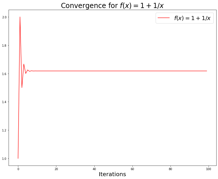

# 
# fixed-point
fp = vals[-1]; fp

1.618033988749895

def f2(x):
  return 1 + 1/x

f2(fp)

1.618033988749895

# 
# x = f(x)
f2(f2(f2(f2(f2(f2(f2(f2(f2(f2(f2(f2(f2(fp)))))))))))))

1.618033988749895

3.2.2 Example 2: $f(x)=cos(x)$

Let’s now use this function on the second example:

x = 0.0
gen = iterate(step=lambda y: np.cos(y), start=x); gen

<generator object iterate at 0x7f99ecd48050>

vals = [next(gen) for i in range(100)]; #vals

fig,axs = plt.subplots(figsize=(13,10))
axs.set_xlabel('Iterations', fontsize=20)
axs.set_title(f'Convergence for $f(x) = cos(x)$', fontsize=24)
axs.plot(vals, color='r', label='$f(x)=cos(x)$')
axs.legend(fontsize=20);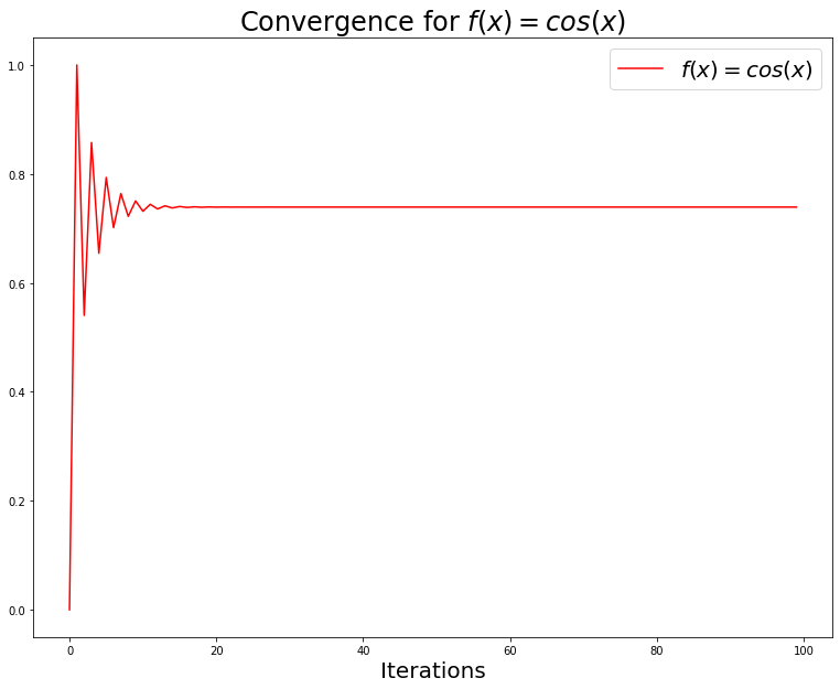

# 
# fixed-point
fp = vals[-1]; fp

0.7390851332151607

np.cos(fp)

0.7390851332151607

# 
# x = f(x)
np.cos(np.cos(np.cos(np.cos(np.cos(np.cos(np.cos(np.cos(np.cos(fp)))))))))

0.7390851332151607

3.3 converge function

The iterate function provides an endless stream of values. It would be nice to wrap it with another function that can specify the criterium for convergence so that the iteration can stop based on this criterium rather than a pre-specified number of iterations.

Let’s call such a function converge():

def converge(values: Iterator[X], done: Callable[[X, X], bool]) -> Iterator[X]:
    '''Read values from an iterator until two consecutive values satisfy the
    given done function or the input iterator ends.
    '''
    a = next(values, None)
    if a is None:
        return
    yield a
    for b in values:
        yield b
        if done(a, b):
            return
        a = b

The converge() function has the inputs: - values: the values generated by the iterate function - done: a function that returns True if the convergence condition is satisfied

Next we call the converge() function with: - values the iterate() function - done the distance between the two latest values

3.3.1 Example 1: $f(x)=1+1/x$

x = 1.0
values = converge(
  values=iterate(lambda y: 1 + 1/y, x),
  done=lambda a, b: np.abs(a-b) < 1e-3
)

# 
# convert values iterator to a list
vals = list(values); vals

[1.0,
 2.0,
 1.5,
 1.6666666666666665,
 1.6,
 1.625,
 1.6153846153846154,
 1.619047619047619,
 1.6176470588235294,
 1.6181818181818182]

fig,axs = plt.subplots(figsize=(13,10))
axs.set_xlabel('Iterations', fontsize=20)
axs.set_title(f'Convergence for $f(x) = 1 + 1/x$', fontsize=24)
axs.plot(vals, color='r', label='$f(x)=1 + 1/x$')
axs.legend(fontsize=20);

3.3.2 Example 2: $f(x)=cos(x)$

x = 0.0
values = converge(
  values=iterate(lambda y: np.cos(y), x),
  done=lambda a, b: np.abs(a-b) < 1e-3
)

# 
# convert values iterator to a list
vals = list(values); vals

[0.0,
 1.0,
 0.5403023058681398,
 0.8575532158463934,
 0.6542897904977791,
 0.7934803587425656,
 0.7013687736227565,
 0.7639596829006542,
 0.7221024250267077,
 0.7504177617637605,
 0.7314040424225098,
 0.7442373549005569,
 0.7356047404363474,
 0.7414250866101092,
 0.7375068905132428,
 0.7401473355678757,
 0.7383692041223232,
 0.7395672022122561,
 0.7387603198742113]

fig,axs = plt.subplots(figsize=(13,10))
axs.set_xlabel('Iterations', fontsize=20)
axs.set_title(f'Convergence for $f(x) = cos(x)$', fontsize=24)
axs.plot(vals, color='r', label='$f(x)=cos(x)$')
axs.legend(fontsize=20);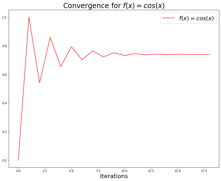

3.4 converged function

The converge() function returns an iterator. It would be nice if we wrap this function even more to just return the final converged value. We also need a last() function to extract the last value of the iteration.

def last(values: Iterator[X]) -> Optional[X]:
    '''Return the last value of the given iterator.
    '''
    try:
        *_, last_element = values
        return last_element
    except ValueError:
        return None

def converged(values: Iterator[X],
              done: Callable[[X, X], bool]) -> X:
    '''Return the final value of the given iterator after its values have
    converged subject to the done function.
    '''
    result = last(converge(values, done))
    if result is None:
        raise ValueError("converged called on an empty iterator")
    return result

3.4.1 Example 1: $f(x)=1+1/x$

x = 1.0
converged_value = converged(
  values=iterate(lambda y: 1 + 1/y, x),
  done=lambda a, b: np.abs(a-b) < 1e-3
)
converged_value

1.6181818181818182

3.4.2 Example 2: $f(x)=cos(x)$

x = 0.0
converged_value = converged(
  values=iterate(lambda y: np.cos(y), x),
  done=lambda a, b: np.abs(a-b) < 1e-3
)
converged_value

0.7387603198742113

3.5 values_provider_ and almost_equal_ functions

Finally, it would be nice if we wrap the iterate function with a values_provider function that includes the function $f(x)$. It could also accept some parameters that might be used in $f(x)$. Each use case will likely have its own version of this function.

We can also wrap the function that provides the convergence test, which will be called almost_equal_floats.

3.5.1 Example 1: $f(x)=1+1/x$

def values_provider_example1(a: float) -> Iterator[float]:
  def update(x: float) -> float:
    return a + a/x
  x_0 = 1.0
  return iterate(update, x_0)

def almost_equal_floats_example1(a: float, b: float) -> bool:
  return np.abs(a-b) < 1e-3

converged_value = converged(
  values=values_provider_example1(a=1),
  done=almost_equal_floats_example1
)
converged_value

1.6181818181818182

3.5.2 Example 2: $f(x)=cos(x)$

def values_provider_example2() -> Iterator[float]:
  def update(x: float) -> float:
    return np.cos(x)
  x_0 = 0.0
  return iterate(update, x_0)

def almost_equal_floats_example2(a: float, b: float) -> bool:
  return np.abs(a-b) < 1e-3

converged_value = converged(
  values=values_provider_example2(),
  done=almost_equal_floats_example2
)
converged_value

0.7387603198742113