! python --versionPython 3.11.14In this project we establish an Active Inference (AIF) modeling approach making use of Bond Graphs, Generalized Filters, and Generalized Coordinates of Motion for traditional engineering systems. The emphasis will be on creating a framework and methodology, rather than applying it to a substantial problem. In this first part, we will make use of Bond Graphs to derive the state space equations that will be used in the following parts.
A few coding conventions:
! python --versionPython 3.11.14import BondGraphTools as bgt
from BondGraphTools import component_manager as cm
import importlib.metadata as md
import sympy as sp
import matplotlib.pyplot as plt
import numpy as np
from scipy.integrate import solve_ivp
from matplotlib.gridspec import GridSpec
from IPython.display import Math, display
print("BondGraphTools:", md.version("BondGraphTools"))
print("sympy:", sp.__version__)BondGraphTools: 0.4.6
sympy: 1.14.0The current need is to establish an Active Inference (AIF) modeling approach making use of Bond Graphs, Generalized Filters, and Generalized Coordinates of Motion for traditional engineering systems. The emphasis will be on creating a framework and methodology, rather than applying it to a substantial problem. In this first part, we will make use of Bond Graphs to derive the state space equations that will be used in the following parts.
Bond graphs provide an energy-based, domain-independent way to derive state-space models that is especially useful for complex, multi-physics engineering systems. They turn the messy bookkeeping of variables and interconnections into a structured graphical procedure for obtaining first-order equations in a systematic way.
Using bond graphs, engineers can:
- Work with a unified representation across mechanical, electrical, thermal and other domains, which simplifies deriving coupled state-space equations for multi-domain systems.
- Exploit causality assignment to automatically identify suitable state variables (typically energy storage variables) and algorithmically generate consistent state-space or differential-algebraic equations.
- Gain physical insight into power flow, storage and dissipation, which helps validate models, anticipate structural properties (e.g. controllability issues), and support modular model reuse and extension.
Generalized filtering provides a variational Bayesian framework for estimating and controlling the hidden states of nonlinear dynamical systems in continuous time. By formulating inference as gradient descent on a free-energy functional, it delivers online state and parameter estimates that can be directly coupled to control laws, without the need for backward passes as in standard smoothing approaches.
When applied to systems whose state equations are derived from bond graphs, generalized filters operate on physically meaningful energy-based state variables, allowing control to respect the underlying power flows and conservation laws encoded in the model. This combination enables a principled closed-loop scheme in which bond-graph state equations generate predictions, generalized filtering updates beliefs about hidden states and disturbances, and control actions are optimized by minimizing variational free energy—effectively unifying estimation and control within a single coherent formalism.
Our current system consists of a single room which temperature needs to be controlled, given a setpoint function. The outside temperature serves as a disturbance and an HVAC system implements the control signal.
To derive the state equations we will make use of bondgraph modeling. Instead of considering the displacement of entropy \(S\) and using entropy flow \(\dot S\) for a flow variable, we will make use of a thermal pseudo-bondgraph. This allows us to consider the displacement of heat \(Q\) and use \(\dot Q\) for a flow variable. The latter arrangement is more popular in the area of thermal control. The next diagram shows a network of bondgraph components as well as the associated bondgraph.
from IPython.display import Image, display
display(Image(filename="ThermicSystem-BG.png"))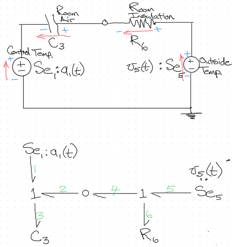
print("Libraries:")
for lib_id, lib_desc in cm.get_library_list():
    print(f"- {lib_id}: {lib_desc}")

print("\nElements in each library:")
for lib_id, lib_desc in cm.get_library_list():
    print(f"\n[{lib_id}] {lib_desc}")
    comps = cm.get_components_list(lib_id)
    for cid, desc in comps:
        print(f"  {cid:10s}  {desc}")
Libraries:
- elec: Electrical Components
- BioChem: Biochemical Components
- base: Basic Components
Elements in each library:
[elec] Electrical Components
Di Diode
BJT Bipolar Junction Transistor
[BioChem] Biochemical Components
Ce Concentration of Chemical Species
Re Biochemical Reaction
Y Stoichiometry
[base] Basic Components
0 Equal Effort Node
1 Equal Flow Node
R Generalised Linear Resistor
C Generalised Linear Capacitor
I Generalised Linear Inductor
Se Effort Source
Sf Flow Source
TF Linear Transformer
GY Linear Gyrator
SS Source Sensor
PH Port Hamiltonianbg = bgt.new(name="Thermic System")Se1_sym, C3_sym, R6_sym, Se5_sym = \
sp.symbols('Se1 C3 R6 Se5') ## names
Se1 = bgt.new(component='Se', name='Se1', value=Se1_sym)
_1_123 = bgt.new(component='1', name='_1_123')
C3 = bgt.new(component='C', name='C3', value=C3_sym)
_0_24 = bgt.new(component='0', name='_0_24')
_1_456 = bgt.new(component='1', name='_1_456')
R6 = bgt.new(component='R', name='R6', value=R6_sym)
Se5 = bgt.new(component='Se', name='Se5', value=Se5_sym)bgt.add(bg, Se1, _1_123, C3, _0_24, _1_456, R6, Se5)bgt.connect(Se1, _1_123)
bgt.connect(_1_123, C3)
bgt.connect(_0_24, _1_123)
bgt.connect(_1_456, _0_24)
bgt.connect(_1_456, R6)
bgt.connect(Se5, _1_456)bgt.draw(bg)
plt.show()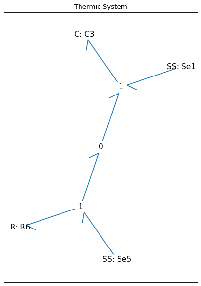
print("State vars:", bg.state_vars); print()
for i,rel in enumerate(bg.constitutive_relations):
print(i, rel)State vars: {'x_0': (C: C3, 'q_0')}
0 dx_0 - Se1/R6 - Se5/R6 + x_0/(C3*R6)print("State vars:", bg.state_vars); print()
for i,rel in enumerate(bg.constitutive_relations):
print(i, rel)
print()
## internal names (from BondGraphTools)
x0 = sp.symbols('x_0')
dx0 = sp.symbols('dx_0')
Se1 = sp.symbols('Se1')
Se5 = sp.symbols('Se5')
## external preferred names
q3 = sp.symbols('q3')
dq3 = sp.symbols('dq3')
a1 = sp.symbols('a1(t)')
v5 = sp.symbols('v5(t)')
subs_map = {
x0: q3,
dx0: dq3,
Se1: a1,
Se5: v5
}
relabeled = [rel.subs(subs_map) for rel in bg.constitutive_relations]
for i,r in enumerate(relabeled):
print(i, r)State vars: {'x_0': (C: C3, 'q_0')}
0 dx_0 - Se1/R6 - Se5/R6 + x_0/(C3*R6)
0 dq3 - a1(t)/R6 - v5(t)/R6 + q3/(C3*R6)def simplify_for_state_space(sol):
sol_terms = sp.expand(sol); display(Math(sp.latex(sol_terms))) ## needed even when next statement is used
terms = sol_terms.as_ordered_terms(); display(Math(sp.latex(terms))) ## list of terms in the sum
simplified_terms = []
for term in terms:
## Get numerator and denominator of this term
num, den = sp.fraction(term)
## Factor numerator and denominator
num_f = sp.factor(num)
den_f = sp.factor(den)
## Cancel common factors within this term
term_simpl = sp.cancel(num_f / den_f)
simplified_terms.append(term_simpl)
## Recombine simplified terms into a single expression
expr_simpl = sp.Add(*simplified_terms); display(Math(sp.latex(expr_simpl)))
return expr_simpl
def simplify_final_terms(ex):
terms2 = ex.as_ordered_terms(); display(Math(sp.latex(terms2)))
simplified_terms2 = []
for term2 in terms2:
term_simpl2 = sp.simplify(term2)
simplified_terms2.append(term_simpl2)
expr_simpl2 = sp.Add(*simplified_terms2); display(Math(sp.latex(expr_simpl2)))
return expr_simpl2## setup symbols for solver
C3, R6 = sp.symbols('C3 R6')
t = sp.symbols('t')
a1 = sp.Function('a1')
v5 = sp.Function('v5')## solve for dq3
## 0:
expr = dq3 - a1(t)/R6 - v5(t)/R6 + q3/(C3*R6)
eq = sp.Eq(expr, 0)
sol = sp.solve(eq, dq3)[0]
ex = simplify_for_state_space(sol)
## ex = sp.collect(ex, [F(t)]); display(Math(sp.latex(ex)))
ex = simplify_final_terms(ex)
## ex = ex.as_ordered_terms()
## sp.factor(sp.denom(ex[0]))\(\displaystyle \frac{a_{1}{\left(t \right)}}{R_{6}} + \frac{v_{5}{\left(t \right)}}{R_{6}} - \frac{q_{3}}{C_{3} R_{6}}\)
\(\displaystyle \left[ \frac{a_{1}{\left(t \right)}}{R_{6}}, \ \frac{v_{5}{\left(t \right)}}{R_{6}}, \ - \frac{q_{3}}{C_{3} R_{6}}\right]\)
\(\displaystyle \frac{a_{1}{\left(t \right)}}{R_{6}} + \frac{v_{5}{\left(t \right)}}{R_{6}} - \frac{q_{3}}{C_{3} R_{6}}\)
\(\displaystyle \left[ \frac{a_{1}{\left(t \right)}}{R_{6}}, \ \frac{v_{5}{\left(t \right)}}{R_{6}}, \ - \frac{q_{3}}{C_{3} R_{6}}\right]\)
\(\displaystyle \frac{a_{1}{\left(t \right)}}{R_{6}} + \frac{v_{5}{\left(t \right)}}{R_{6}} - \frac{q_{3}}{C_{3} R_{6}}\)
\[ \dot{q}_3(t) = - \frac{1}{C_3 R_6} q_{3}(t) + \frac{1}{R_6}v_5(t) + \frac{1}{R_6}a_1(t) \]
Collect all the equations:
\[ \dot{q}_3(t) = - \frac{1}{C_3 R_6} q_{3}(t) + \frac{1}{R_6}v_5(t) + \frac{1}{R_6}a_1(t) \]
ALPHA = 0.6
ENV_WIDTH = 4. ## 8.
AGT_WIDTH = 2.
AGT_LINESTYLES = ['-', '--', '-.', ':'] ## for agent
ORANGE_HUE_BY_SATURATION = [
"#FFA500", ## 100% bright orange
"#FFB347", ## 80% light vivid orange
"#FFD580", ## 60% softer pastel orange
"#FFE5B4" ## 40% light faded orange
]
ORANGE_HUE_BY_BRIGHTNESS = [
"#FFA500", ## 100% pure bright orange
"#FFC04D", ## 80% light orange
"#FFD699", ## 60% pastel orange
"#FFE5CC" ## 40% very pale orange
]
ORANGE_HUE = ORANGE_HUE_BY_BRIGHTNESS
styles = {
#### envir
"a": {
"color": "crimson",
"linestyle": "-",
"linewidth": ENV_WIDTH,
"alpha": ALPHA
},
"xˣ[0]": {
"color": "black",
"linestyle": "-",
"linewidth": ENV_WIDTH,
"alpha": ALPHA
},
"xˣ[1]": {
"color": "darkgrey",
"linestyle": "-",
"linewidth": ENV_WIDTH,
"alpha": ALPHA
},
"vˣ[0]": {
"color": "blue",
"linestyle": "-",
"linewidth": ENV_WIDTH,
"alpha": ALPHA
},
"vˣ[1]": {
"color": "dodgerblue",
"linestyle": "-",
"linewidth": ENV_WIDTH,
"alpha": ALPHA
},
"y[0]": {
"color": ORANGE_HUE[0],
"linestyle": "-",
"linewidth": ENV_WIDTH,
"alpha": ALPHA
},
"y[1]": {
"color": ORANGE_HUE[1],
"linestyle": "-",
"linewidth": ENV_WIDTH,
"alpha": ALPHA
},
"y[2]": {
"color": ORANGE_HUE[2],
"linestyle": "-",
"linewidth": ENV_WIDTH,
"alpha": ALPHA
},
"y[3]": {
"color": ORANGE_HUE[3],
"linestyle": "-",
"linewidth": ENV_WIDTH,
"alpha": ALPHA
},
#### agent
"μ_x[0]": {
"color": "black",
"linestyle": AGT_LINESTYLES[0],
"linewidth": AGT_WIDTH,
"alpha": ALPHA
},
"μ_x[1]": {
"color": "black",
"linestyle": AGT_LINESTYLES[1],
"linewidth": AGT_WIDTH,
"alpha": ALPHA
},
"v[0]": {
"color": "blue",
"linestyle": AGT_LINESTYLES[0],
"linewidth": AGT_WIDTH,
"alpha": ALPHA
},
"v[1]": {
"color": "blue",
"linestyle": AGT_LINESTYLES[1],
"linewidth": AGT_WIDTH,
"alpha": ALPHA
},
"μ_v[0]": {
"color": "dodgerblue",
"linestyle": AGT_LINESTYLES[0],
"linewidth": AGT_WIDTH,
"alpha": ALPHA
},
"μ_v[1]": {
"color": "dodgerblue",
"linestyle": AGT_LINESTYLES[1],
"linewidth": AGT_WIDTH,
"alpha": ALPHA
},
"μ_y[0]": {
"color": "orange",
"linestyle": AGT_LINESTYLES[0],
"linewidth": AGT_WIDTH,
"alpha": ALPHA
},
"μ_y[1]": {
"color": "orange",
"linestyle": AGT_LINESTYLES[1],
"linewidth": AGT_WIDTH,
"alpha": ALPHA
},
"μ_y[2]": {
"color": "orange",
"linestyle": AGT_LINESTYLES[2],
"linewidth": AGT_WIDTH,
"alpha": ALPHA
},
"F": {
"color": "#9400D3", ## vivid deep violet
"linestyle": "-",
"linewidth": AGT_WIDTH,
"alpha": ALPHA
}
}def plot_states_and_exogvs(
t_span,
t_states,
state_series,
state_labels,
state_styles,
t_exogvs,
exogv_series,
exogv_labels,
exogv_styles,
figsize=(8, 5),
):
"""
state_series: list of 1D arrays (same shape as t_states)
state_labels: list of strings, LaTeX-ready
state_styles: list of dicts, e.g. [styles['xˣ[0]'], styles['xˣ[1]'], ...]
exogv_series: list of 1D arrays (same shape as t_exogvs)
exogv_labels: list of strings
exogv_styles: list of dicts, e.g. [styles['vˣ[0]'], ...]
"""
ylabelx = -0.3
ylabely = 0.3
fig = plt.figure(figsize=figsize)
grid_rows = 2
gs = GridSpec(grid_rows, 1, figure=fig, height_ratios=[1, 1], hspace=0.2)
ax = [fig.add_subplot(gs[i]) for i in range(grid_rows)]
## Common axis formatting
for axis in ax:
axis.grid(True)
axis.spines['top'].set_visible(False)
axis.spines['right'].set_visible(False)
## Top: states
i = 0
ax[i].set_title('states', fontweight='regular', fontsize=12)
for y, lab, st in zip(state_series, state_labels, state_styles):
ax[i].plot(t_states, y, **st, label=lab)
ax[i].set_xticklabels([])
ax[i].yaxis.set_label_coords(ylabelx, ylabely)
ax[i].legend(loc='upper left')
## Bottom: exogvs (exogenous forces)
i = 1
ax[i].set_title('exogenous forces', fontweight='regular', fontsize=12)
for y, lab, st in zip(exogv_series, exogv_labels, exogv_styles):
ax[i].step(t_exogvs, y, where="post", **st, label=lab)
# ax[i].plot(t_exogvs, y, **st, label=lab)
ax[i].legend(loc='upper left')
## X ticks from t_span
x_ticks = np.arange(t_span[0], t_span[1] + 1, 1.0)
ax[i].set_xticks(x_ticks)
ax[i].set_xlabel(r'$\mathrm{Timestep}\ t$', fontweight='bold', fontsize=12)
plt.subplots_adjust(hspace=0.1)
plt.show()
return fig, ax## build values model for simulation
bg = bgt.new(name="Thermic System")
Se1_val = 1.
C3_val = 5.
R6_val = 2.
Se5_val = 1.
Se1 = bgt.new(component='Se', name='Se1', value=Se1_val)
_1_123 = bgt.new(component='1', name='_1_123')
C3 = bgt.new(component='C', name='C3', value=C3_val)
_0_24 = bgt.new(component='0', name='_0_24')
_1_456 = bgt.new(component='1', name='_1_456')
R6 = bgt.new(component='R', name='R6', value=R6_val)
Se5 = bgt.new(component='Se', name='Se5', value=Se5_val)
bgt.add(bg, Se1, _1_123, C3, _0_24, _1_456, R6, Se5)
bgt.connect(Se1, _1_123)
bgt.connect(_1_123, C3)
bgt.connect(_0_24, _1_123)
bgt.connect(_1_456, _0_24)
bgt.connect(_1_456, R6)
bgt.connect(Se5, _1_456)
print(bg.state_vars)
t_span = (0.0, 10.0)
t_eval = np.linspace(t_span[0], t_span[1], 1001)
x0 = [1.] ## initial conditions for C and I states (adjust length if needed){'x_0': (C: C3, 'q_0')}params = {
'C3': C3_val,
'R6': R6_val
}
def make_rhs(v_funcs, params, **v_func_kwargs):
## left sides must be symbols in latex equations
C3 = params['C3']
R6 = params['R6']
## unpack per-source theta dicts, default to empty
v5_theta = v_func_kwargs.get('v5_theta', {})
a1_theta = v_func_kwargs.get('a1_theta', {})
def rhs(t, x):
q3 = x
## exogenous inputs
v5 = v_funcs['v5'](t, **v5_theta)
a1 = v_funcs['a1'](t, **a1_theta)
t1_num = 1; t1_den = C3*R6
t2_num = 1; t2_den = R6
t3_num = 1; t3_den = R6
dq3 = -(t1_num/t1_den)*q3 + (t2_num/t2_den)*v5 + (t3_num/t3_den)*a1
return [dq3]
return rhs
def v_const(t, **kwargs):
# return kwargs['θ1']
return kwargs['A']
def v_cos(t, **kwargs):
return kwargs['A'] * np.cos(kwargs['θ1'] * t)
def v_pulse(t, **kwargs):
return float(kwargs['A']*np.heaviside(t - kwargs['t_up'], 0.0) - kwargs['A']*np.heaviside(t - kwargs['t_down'], 0.0))
def v_pulses(t, **kwargs):
"""
Sum of rectangular pulses defined in physical time.
kwargs:
'amps' : list/array of amplitudes [A1, A2, ...]
't_ons' : list/array of start times [t_on1, t_on2, ...]
't_offs' : list/array of end times [t_off1, t_off2, ...]
"""
amps = np.asarray(kwargs['amps'], dtype=float)
t_ons = np.asarray(kwargs['t_ons'], dtype=float)
t_offs = np.asarray(kwargs['t_offs'], dtype=float)
t_arr = np.asarray(t, dtype=float)
val = np.zeros_like(t_arr, dtype=float)
for A, t_on, t_off in zip(amps, t_ons, t_offs):
val += A * (np.heaviside(t_arr - t_on, 0.0) - np.heaviside(t_arr - t_off, 0.0))
return float(val) if np.isscalar(t) else val
rng = np.random.default_rng(1234)
## --- Option 1: White Gaussian noise with std σ ---
def w_normal(t, **kwargs):
## t can be scalar or array; ignore its value, just match shape
if np.isscalar(t):
return kwargs['A'] * kwargs['sigma'] * rng.normal()
else:
return kwargs['A'] * kwargs['sigma'] * rng.normal(size=np.shape(t))
## --- Option 2: Uniform noise in [-A, A] ---
def w_uniform(t, **kwargs):
## rand in [0,1) → scale/shift to [-A, A]
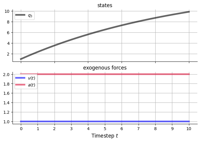
return (2 * kwargs['A']) * (rng.random() - 0.5)v_funcs = {
'v5': v_const,
'a1': v_const,
}
v5_const_A = 1.
a1_const_A = 2.
rhs = make_rhs(
v_funcs,
params,
v5_theta={'A': v5_const_A},
a1_theta={'A': a1_const_A},
)
sol = solve_ivp(rhs, t_span, x0, t_eval=t_eval)
t = sol.t
q3 = sol.y[0] ## x_0
v5_vals = np.vectorize(v_const)(t_eval, A=v5_const_A)
a1_vals = np.vectorize(v_const)(t_eval, A=a1_const_A)
fig, ax = plot_states_and_exogvs(
t_span=t_span,
t_states=t,
state_series=[q3],
state_labels=[
r'$q_{3}$'
],
state_styles=[
styles['xˣ[0]']
],
t_exogvs=t_eval,
exogv_series=[v5_vals, a1_vals],
exogv_labels = [r'$v(t)$', r'$a(t)$'],
exogv_styles=[styles['vˣ[0]'], styles['a']],
)
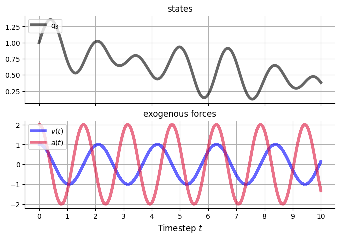
v_funcs = {
    'v5':  v_cos,
    'a1':  v_cos,
}
v5_cos_A = 1.
v5_cos_θ1 = 3.
a1_cos_A = 2.
a1_cos_θ1 = 4.
rhs = make_rhs(
    v_funcs,
    params,
    v5_theta={'A': v5_cos_A, 'θ1': v5_cos_θ1},
    a1_theta={'A': a1_cos_A, 'θ1': a1_cos_θ1},
)
sol = solve_ivp(rhs, t_span, x0, t_eval=t_eval)
t = sol.t
q3 = sol.y[0] ## x_0
v5_vals = np.vectorize(v_cos)(t_eval, A=v5_cos_A, θ1=v5_cos_θ1)
a1_vals = np.vectorize(v_cos)(t_eval, A=a1_cos_A, θ1=a1_cos_θ1)

fig, ax = plot_states_and_exogvs(
    t_span=t_span,

    t_states=t,
    state_series=[q3],
    state_labels=[
        r'$q_{3}$'
    ],
    state_styles=[
        styles['xˣ[0]']
    ],

    t_exogvs=t_eval,
    exogv_series=[v5_vals, a1_vals],
    exogv_labels = [r'$v(t)$', r'$a(t)$'],
    exogv_styles=[styles['vˣ[0]'], styles['a']],
)
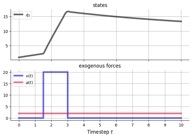
v_funcs = {
    'v5':  v_pulse,
    'a1':  v_const,
}
pulse_A = 20.
pulse_t_up = 1.5
pulse_t_down = 3.
a1_const_A = 2.
rhs = make_rhs(
    v_funcs,
    params,
    v5_theta={'A': pulse_A, 't_up': pulse_t_up, 't_down': pulse_t_down},
    a1_theta={'A': a1_const_A},
)
sol = solve_ivp(rhs, t_span, x0, t_eval=t_eval)
t = sol.t
q3 = sol.y[0] ## x_0
v5_vals = np.vectorize(v_pulse)(t_eval, A=pulse_A, t_up=pulse_t_up, t_down=pulse_t_down)
a1_vals = np.vectorize(v_const)(t_eval, A=a1_const_A)

fig, ax = plot_states_and_exogvs(
    t_span=t_span,

    t_states=t,
    state_series=[q3],
    state_labels=[
        r'$q_{3}$'
    ],
    state_styles=[
        styles['xˣ[0]']
    ],

    t_exogvs=t_eval,
    exogv_series=[v5_vals, a1_vals],
    exogv_labels = [r'$v(t)$', r'$a(t)$'],
    exogv_styles=[styles['vˣ[0]'], styles['a']],
)